Data Mining and machine learning A few important

Data Mining (and machine learning) A few important things in brief top 10 dm, - neural networks – overfitting --- SVM

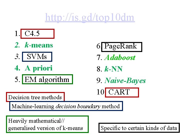
http: //is. gd/top 10 dm 1. 2. 3. 4. 5. C 4. 5 k-means SVMs A priori EM algorithm 6. Page. Rank 7. Adaboost 8. k-NN 9. Naive-Bayes 10. CART

http: //is. gd/top 10 dm 1. 2. 3. 4. 5. C 4. 5 k-means SVMs A priori EM algorithm 6. Page. Rank 7. Adaboost 8. k-NN 9. Naive-Bayes 10. CART The 10 most mentioned in Data Mining academic literature up to 2007, not including Machine Learning literature

http: //is. gd/top 10 dm 1. 2. 3. 4. 5. C 4. 5 k-means SVMs A priori EM algorithm 6. Page. Rank 7. Adaboost 8. k-NN 9. Naive-Bayes 10. CART

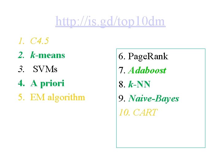
http: //is. gd/top 10 dm 1. 2. 3. 4. 5. C 4. 5 k-means SVMs A priori EM algorithm 6. Page. Rank 7. Adaboost 8. k-NN 9. Naive-Bayes 10. CART Decision tree methods Machine-learning decision boundary method Heavily mathematical// generalised version of k-means Specific to certain kinds of data

So. . . Today we will look at: The no. 1 Machine Learning method … Overfitting (this is a good place for it. . . ) Support vector machines in the last lecture we will see the new number 1 Machine learning method …

Decision boundary methods: finding a separating boundary

Decision boundary methods: finding a separating boundary

Decision boundary methods: finding a separating boundary

Decision boundary methods: finding a separating boundary

Decision boundary methods: finding a separating boundary

Decision boundary methods: finding a separating boundary

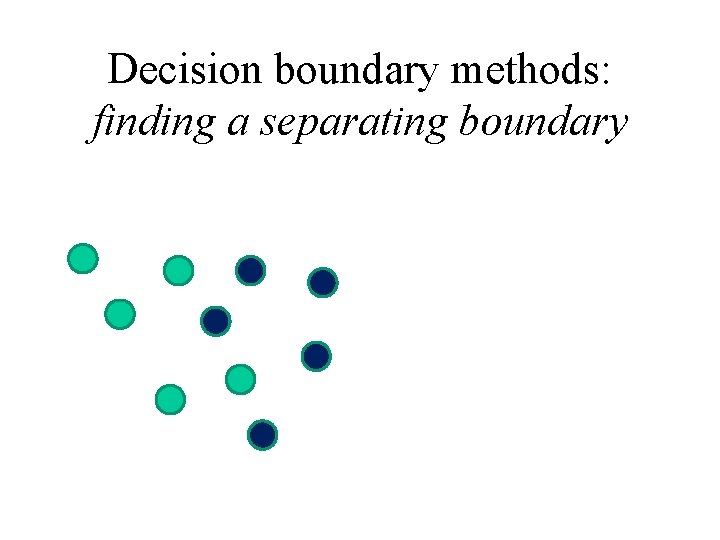
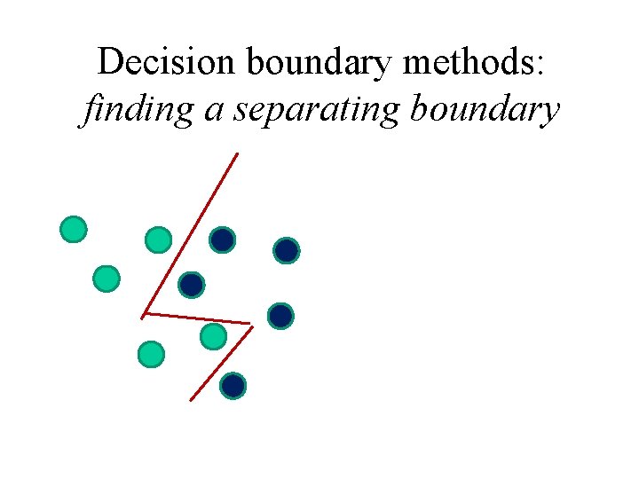
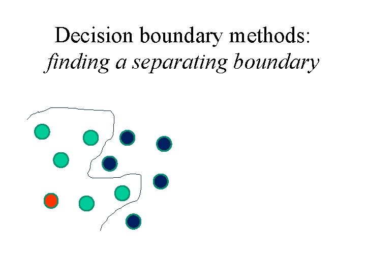
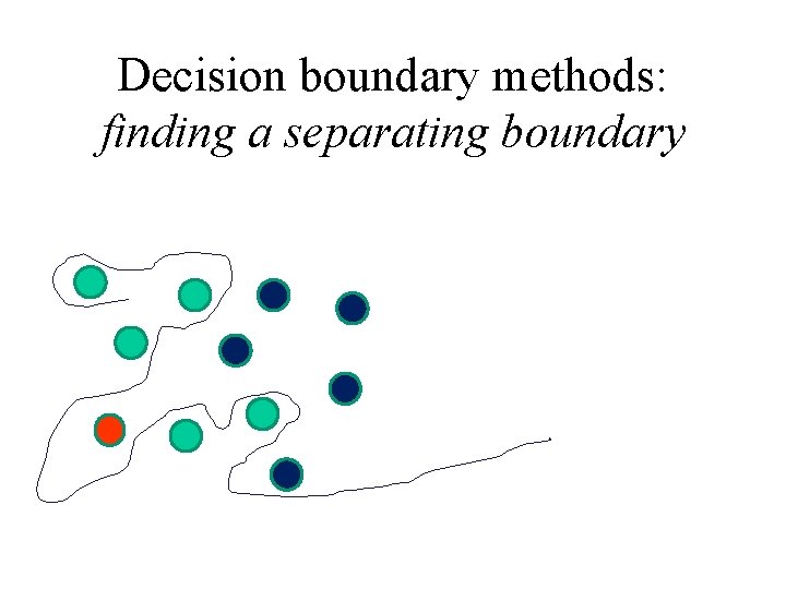
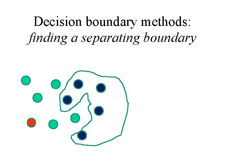
If your data were 2 D, you could plot your known data points, colour with known classes and draw the boundary you think looks best, and use that as the classifier

If your data were 2 D, you could plot your known data points, colour with known classes and draw the boundary you think looks best, and use that as the classifier But it’s much more common (and effective) to use machine learning methods. Neural Networks and Support Vector Machines are the most common ‘decision boundary’ methods. In both cases they learn by finding the parameters for a very complex curve – and that’s the decision boundary.

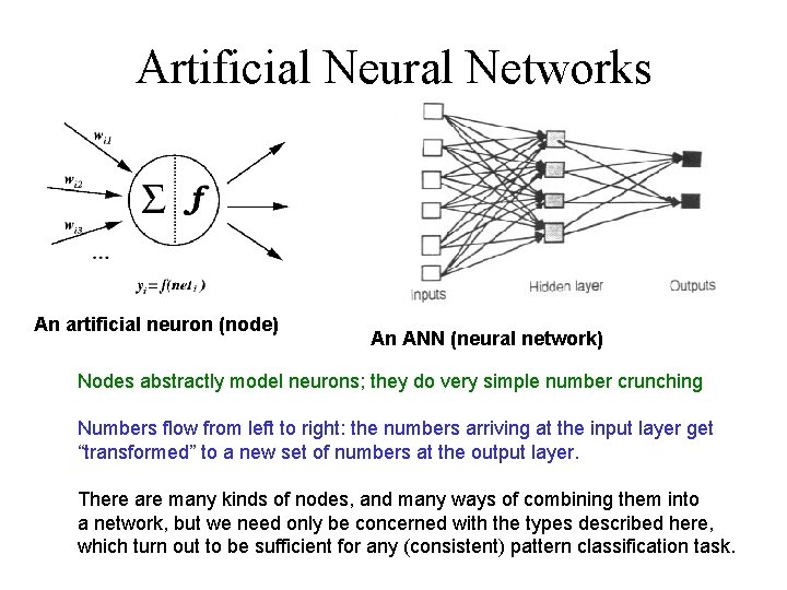
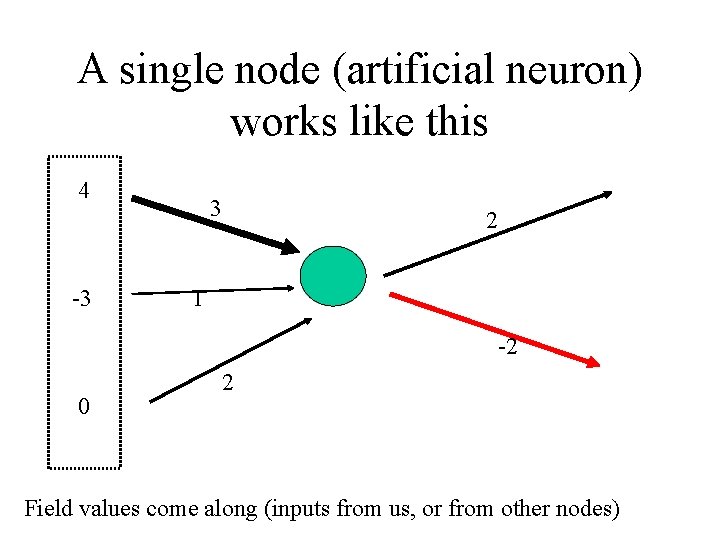
Artificial Neural Networks An artificial neuron (node) An ANN (neural network) Nodes abstractly model neurons; they do very simple number crunching Numbers flow from left to right: the numbers arriving at the input layer get “transformed” to a new set of numbers at the output layer. There are many kinds of nodes, and many ways of combining them into a network, but we need only be concerned with the types described here, which turn out to be sufficient for any (consistent) pattern classification task.

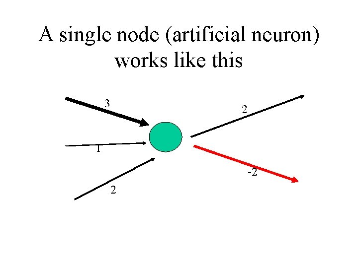
A single node (artificial neuron) works like this 3 2 1 -2 2

A single node (artificial neuron) works like this 4 -3 3 2 1 -2 0 2 Field values come along (inputs from us, or from other nodes)

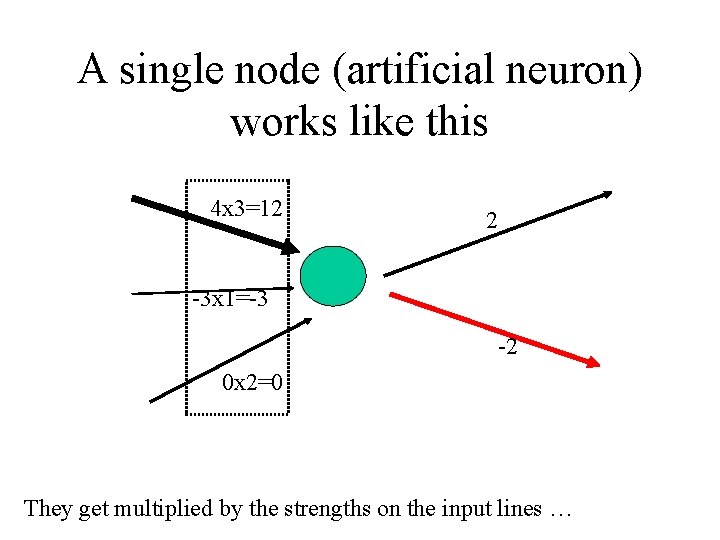
A single node (artificial neuron) works like this 4 x 3=12 2 -3 x 1=-3 -2 0 x 2=0 They get multiplied by the strengths on the input lines …

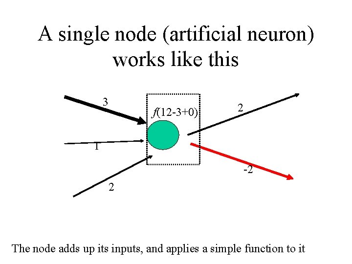
A single node (artificial neuron) works like this 3 f(12 -3+0) 2 1 -2 2 The node adds up its inputs, and applies a simple function to it

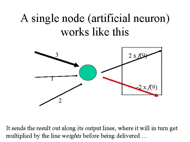
A single node (artificial neuron) works like this 3 2 x f(9) 1 -2 x f(9) 2 It sends the result out along its output lines, where it will in turn get multiplied by the line weights before being delivered …

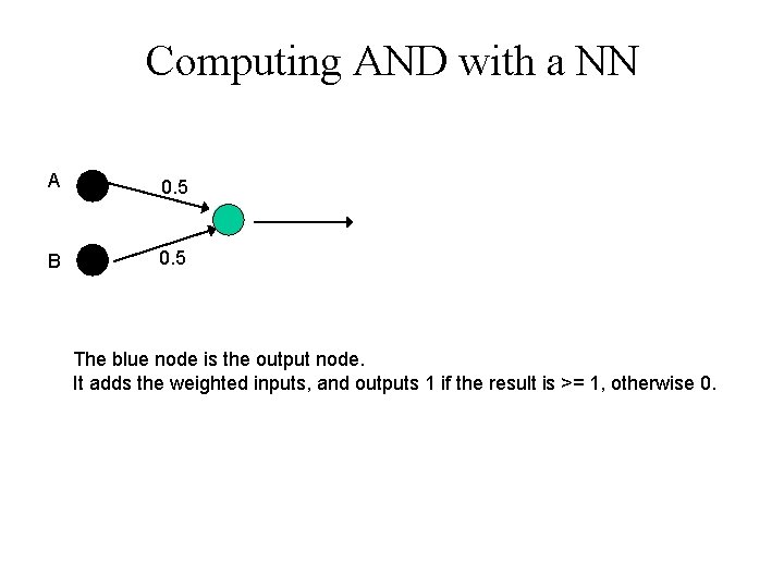
Computing AND with a NN A 0. 5 B 0. 5 The blue node is the output node. It adds the weighted inputs, and outputs 1 if the result is >= 1, otherwise 0.

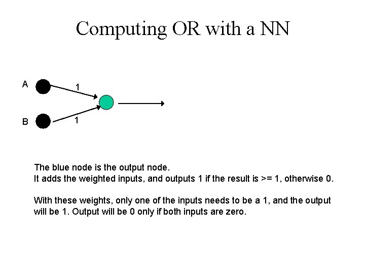
Computing OR with a NN A 1 B 1 The blue node is the output node. It adds the weighted inputs, and outputs 1 if the result is >= 1, otherwise 0. With these weights, only one of the inputs needs to be a 1, and the output will be 1. Output will be 0 only if both inputs are zero.

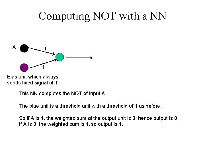
Computing NOT with a NN A -1 1 Bias unit which always sends fixed signal of 1 This NN computes the NOT of input A The blue unit is a threshold unit with a threshold of 1 as before. So if A is 1, the weighted sum at the output unit is 0, hence output is 0; If A is 0, the weighted sum is 1, so output is 1.

So, an NN can compute AND, OR and NOT – so what? It is straightforward to combine ANNs together, with outputs from some becoming the inputs of others, etc. That is, we can combine them just like logic gates on a microchip. And this means that a neural network can compute ANY function of the inputs

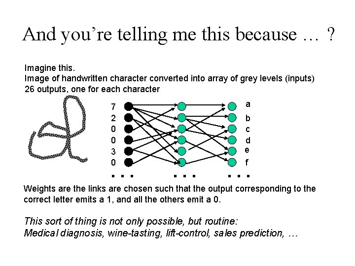
And you’re telling me this because … ? Imagine this. Image of handwritten character converted into array of grey levels (inputs) 26 outputs, one for each character 7 2 0 0 3 0 … a b c d e f … … Weights are the links are chosen such that the output corresponding to the correct letter emits a 1, and all the others emit a 0. This sort of thing is not only possible, but routine: Medical diagnosis, wine-tasting, lift-control, sales prediction, …

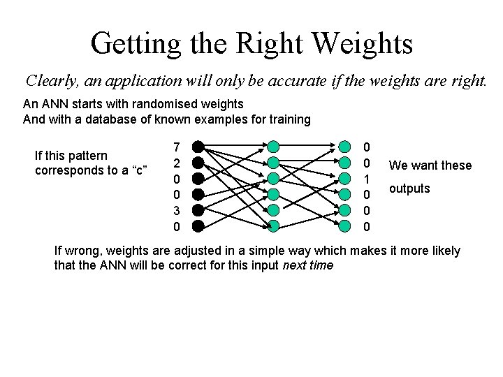
Getting the Right Weights Clearly, an application will only be accurate if the weights are right. An ANN starts with randomised weights And with a database of known examples for training If this pattern corresponds to a “c” 7 2 0 0 3 0 0 0 1 0 0 0 We want these outputs If wrong, weights are adjusted in a simple way which makes it more likely that the ANN will be correct for this input next time

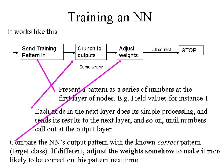
Training an NN It works like this: Send Training Pattern in Crunch to outputs Adjust weights All correct STOP Some wrong Present a pattern as a series of numbers at the first layer of nodes. E. g. Field values for instance 1 Each node in the next layer does its simple processing, and sends its results to the next layer, and so on, until numbers call out at the output layer Compare the NN’s output pattern with the known correct pattern (target class). If different, adjust the weights somehow to make it more likely to be correct on this pattern next time.

`Classical’ NN Training An algorithm called backpropagation BP is the classic way of training a neural network. Based on partial differentiation, it prescribes a way to adjust the weights so that the error on the latest pattern would probably be reduced next time. We can instead use any optimisation algorihm(e. g. GA) to find the weights for a NN. E. g. the first ever significant application of particle swarm optimisation, showed that it was faster than BP, with better results.

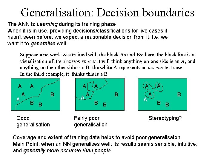
Generalisation: Decision boundaries The ANN is Learning during its training phase When it is in use, providing decisions/classifications for live cases it hasn’t seen before, we expect a reasonable decision from it. I. e. we want it to generalise well. Suppose a network was trained with the black As and Bs; here, the black line is a visualisation of it’s decision space; it will think anything on one side is an A, and anything on the other side is a B. the white A represents an unseen test case. In the third example, it thinks this is a B A A A B B B Good generalisation A A B B B Fairly poor generalisation A A A B B B Stereotyping? Coverage and extent of training data helps to avoid poor generalisaton Main Point: when an NN generalises well, its results seems sensible, intuitive, and generally more accurate than people

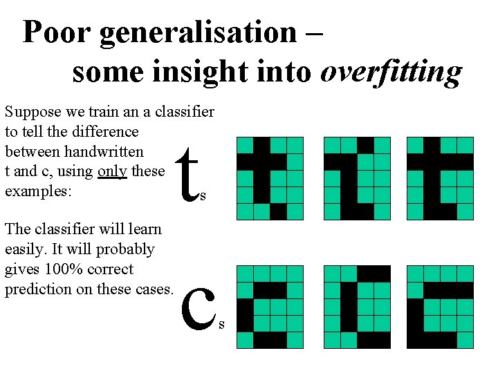
Poor generalisation – some insight into overfitting Suppose we train an a classifier to tell the difference between handwritten t and c, using only these examples: s The classifier will learn easily. It will probably gives 100% correct prediction on these cases. t c s

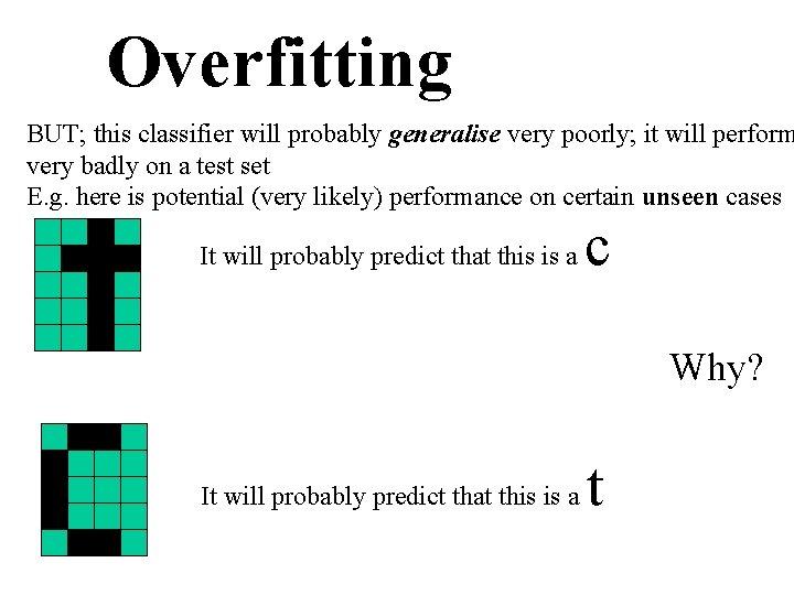
Overfitting BUT; this classifier will probably generalise very poorly; it will perform very badly on a test set E. g. here is potential (very likely) performance on certain unseen cases It will probably predict that this is a c Why? It will probably predict that this is a t

Avoiding Overfitting It can be avoided by using as much training data as possible, ensuring as much diversity as possible in the data. This cuts down on the potential existence of features that might be discriminative in the training data, but are otherwise spurious. It can be avoided by jittering (adding noise). During training, every time an input pattern ispresented, it is randomly perturbed. The idea of this is that spurious features will be `washed out’ by the noise, but valid discriminatory features will remain. The problem with this approach is how to correctly choose the level of noise.

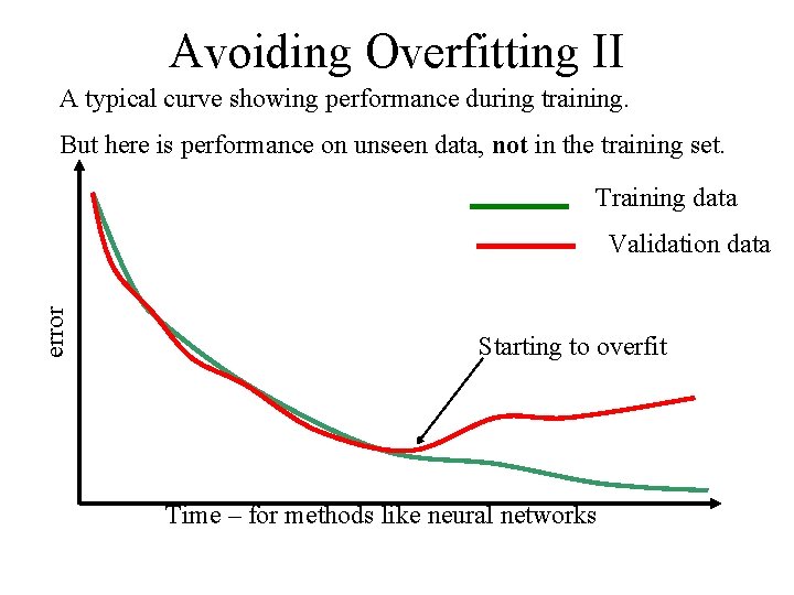
Avoiding Overfitting II A typical curve showing performance during training. But here is performance on unseen data, not in the training set. Training data error Validation data Starting to overfit Time – for methods like neural networks

Avoiding Overfitting III Another approach is early stopping. During training, keep track of the network’s performance on a separate validation set of data. At the point where error continues to improve on the training set, but starts to get worse on the validation set, that is when training should be stopped, since it is starting to overfit on the training data. The problem here is that this point is far from always clear cut.

Real-world applications of ANNs are all over the place

Stocks, Commodities and Futures Currency Price Predictions James O'Sullivan: Controls trading of more than 10 different financial markets with consistent profits. Corporate Bond Rating George Pugh: Predicts corporate bond ratings with 100% accuracy for consulting and trading. Standard and Poor's 500 Prediction LBS Capital Management, Inc: Predicts the S&P 500 one day ahead and one week ahead with better accuracy than traditional methods. Forecasting Stock Prices Walkrich Investments: Neural Networks rate underpriced stock; beating the S&P.

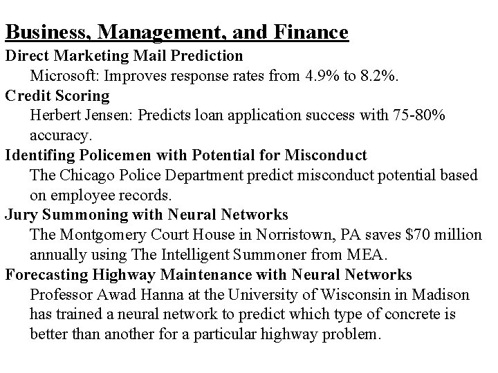
Business, Management, and Finance Direct Marketing Mail Prediction Microsoft: Improves response rates from 4. 9% to 8. 2%. Credit Scoring Herbert Jensen: Predicts loan application success with 75 -80% accuracy. Identifing Policemen with Potential for Misconduct The Chicago Police Department predict misconduct potential based on employee records. Jury Summoning with Neural Networks The Montgomery Court House in Norristown, PA saves $70 million annually using The Intelligent Summoner from MEA. Forecasting Highway Maintenance with Neural Networks Professor Awad Hanna at the University of Wisconsin in Madison has trained a neural network to predict which type of concrete is better than another for a particular highway problem.

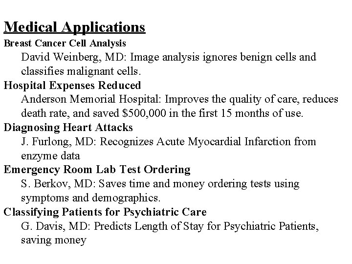
Medical Applications Breast Cancer Cell Analysis David Weinberg, MD: Image analysis ignores benign cells and classifies malignant cells. Hospital Expenses Reduced Anderson Memorial Hospital: Improves the quality of care, reduces death rate, and saved $500, 000 in the first 15 months of use. Diagnosing Heart Attacks J. Furlong, MD: Recognizes Acute Myocardial Infarction from enzyme data Emergency Room Lab Test Ordering S. Berkov, MD: Saves time and money ordering tests using symptoms and demographics. Classifying Patients for Psychiatric Care G. Davis, MD: Predicts Length of Stay for Psychiatric Patients, saving money

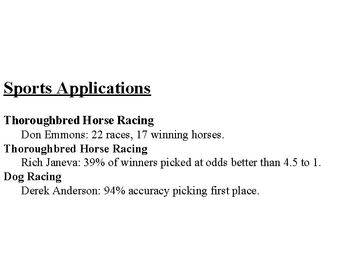
Sports Applications Thoroughbred Horse Racing Don Emmons: 22 races, 17 winning horses. Thoroughbred Horse Racing Rich Janeva: 39% of winners picked at odds better than 4. 5 to 1. Dog Racing Derek Anderson: 94% accuracy picking first place.

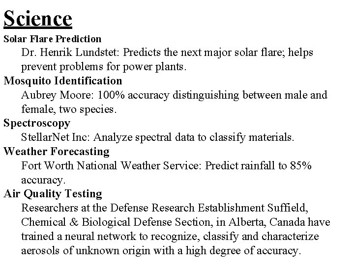
Science Solar Flare Prediction Dr. Henrik Lundstet: Predicts the next major solar flare; helps prevent problems for power plants. Mosquito Identification Aubrey Moore: 100% accuracy distinguishing between male and female, two species. Spectroscopy Stellar. Net Inc: Analyze spectral data to classify materials. Weather Forecasting Fort Worth National Weather Service: Predict rainfall to 85% accuracy. Air Quality Testing Researchers at the Defense Research Establishment Suffield, Chemical & Biological Defense Section, in Alberta, Canada have trained a neural network to recognize, classify and characterize aerosols of unknown origin with a high degree of accuracy.

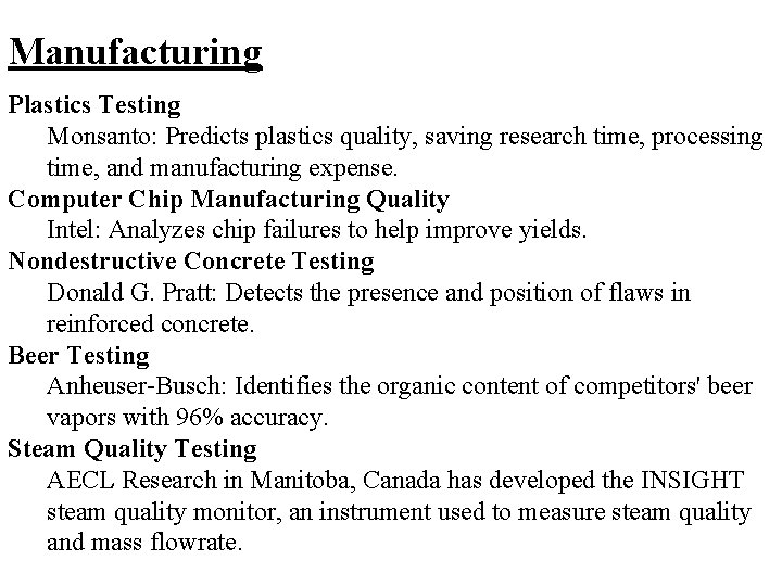
Manufacturing Plastics Testing Monsanto: Predicts plastics quality, saving research time, processing time, and manufacturing expense. Computer Chip Manufacturing Quality Intel: Analyzes chip failures to help improve yields. Nondestructive Concrete Testing Donald G. Pratt: Detects the presence and position of flaws in reinforced concrete. Beer Testing Anheuser-Busch: Identifies the organic content of competitors' beer vapors with 96% accuracy. Steam Quality Testing AECL Research in Manitoba, Canada has developed the INSIGHT steam quality monitor, an instrument used to measure steam quality and mass flowrate.

Support Vector Machines: a different approach to finding the decision surface, particularly good at generalisation

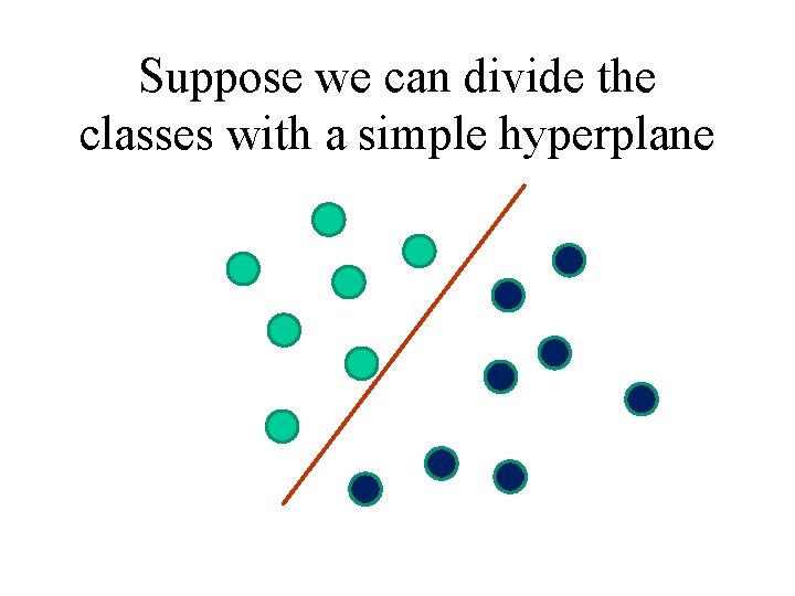
Suppose we can divide the classes with a simple hyperplane

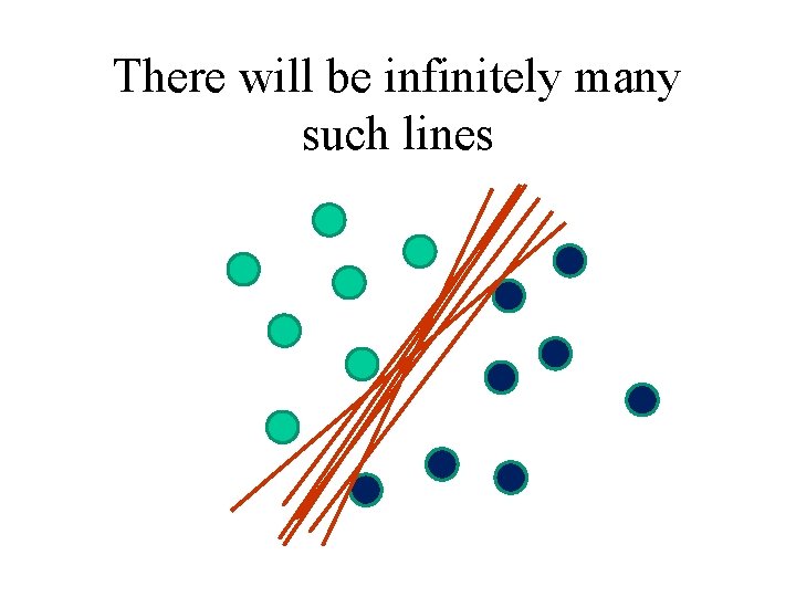
There will be infinitely many such lines

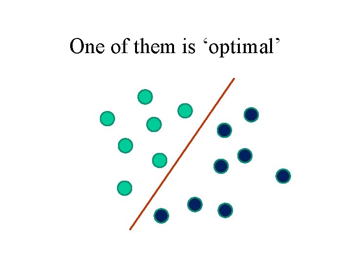
One of them is ‘optimal’

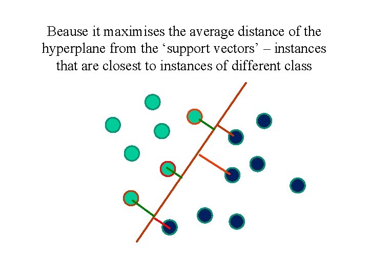
Beause it maximises the average distance of the hyperplane from the ‘support vectors’ – instances that are closest to instances of different class

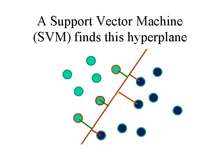
A Support Vector Machine (SVM) finds this hyperplane

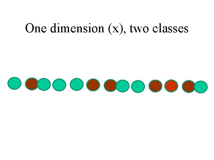
But, usually there is no simple hyperplane that separates the classes!

One dimension (x), two classes

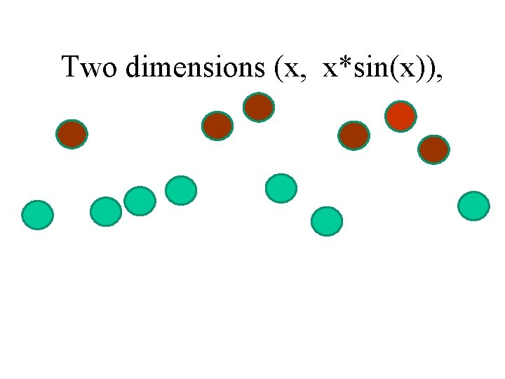
Two dimensions (x, x*sin(x)),

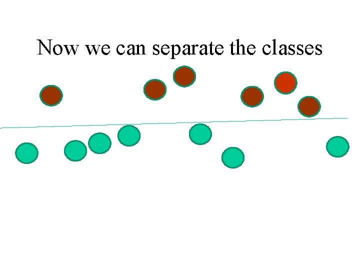
Now we can separate the classes

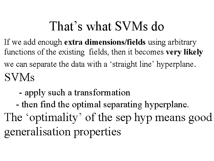
That’s what SVMs do If we add enough extra dimensions/fields using arbitrary functions of the existing fields, then it becomes very likely we can separate the data with a ‘straight line’ hyperplane. SVMs - apply such a transformation - then find the optimal separating hyperplane. The ‘optimality’ of the sep hyp means good generalisation properties

Next: the classic, field-defining DM algorithm