Data Mining and Knowledge Acquizition Chapter 5 BIS

Data Mining: and Knowledge Acquizition — Chapter 5 — BIS 541 2016/2017 Summer 1

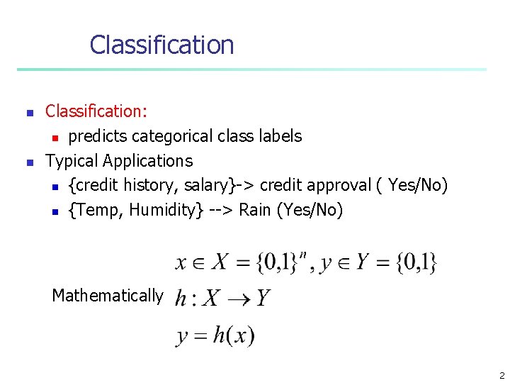
Classification n n Classification: n predicts categorical class labels Typical Applications n {credit history, salary}-> credit approval ( Yes/No) n {Temp, Humidity} --> Rain (Yes/No) Mathematically 2

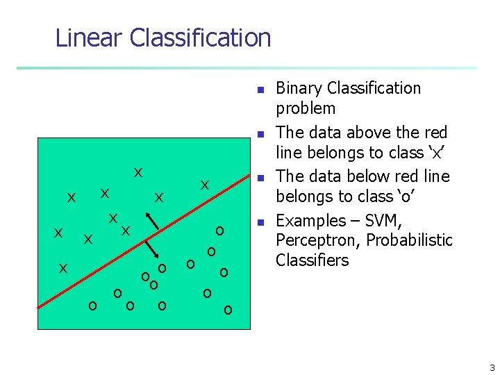
Linear Classification n n x x x x x ooo o o x o o o n n Binary Classification problem The data above the red line belongs to class ‘x’ The data below red line belongs to class ‘o’ Examples – SVM, Perceptron, Probabilistic Classifiers 3

Neural Networks n Analogy to Biological Systems (Indeed a great example of a good learning system) n Massive Parallelism allowing for computational efficiency n The first learning algorithm came in 1959 (Rosenblatt) who suggested that if a target output value is provided for a single neuron with fixed inputs, one can incrementally change weights to learn to produce these outputs using the perceptron learning rule 4

Neural Networks n n Advantages n prediction accuracy is generally high n robust, works when training examples contain errors n output may be discrete, real-valued, or a vector of several discrete or real-valued attributes n fast evaluation of the learned target function Criticism n long training time n difficult to understand the learned function (weights) n not easy to incorporate domain knowledge 5

Network Topology n n Input variables number of inputs number of hidden layers n # of nodes in each hidden layer # of output nodes can handle discrete or continuous variables n normalisation for continuous to 0. . 1 interval n for discrete variables n use k inputs for each level n use k output for each level if k>2 n n A has three distinct values a 1, a 2, a 3 three input variables I 1, I 2 I 3 when A=a 1 I 1=1, I 2, I 3=0 feed-forward: no cycle to input untis fully connected: each unit to each in the forward layer 6

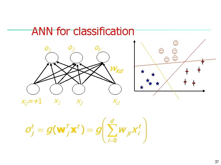
Multi-Layer Perceptron Output vector Output nodes Hidden nodes wij Input nodes Input vector: xi 7

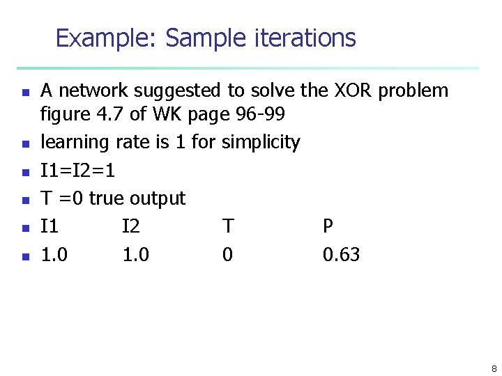
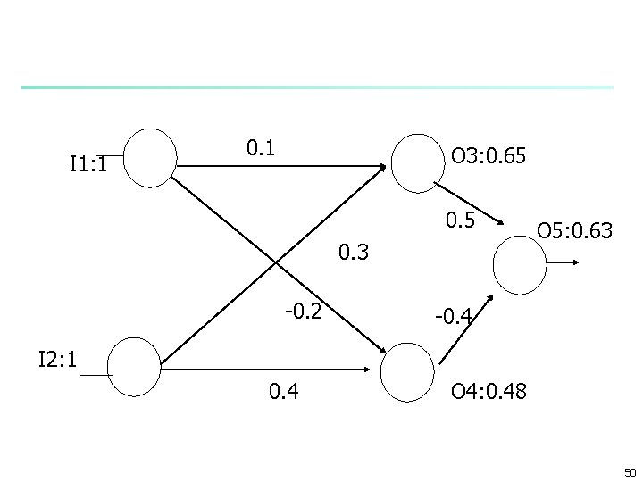
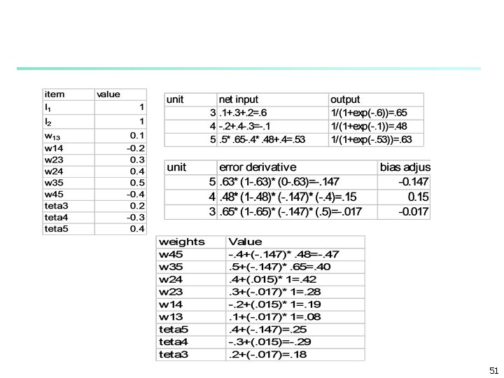
Example: Sample iterations n n n A network suggested to solve the XOR problem figure 4. 7 of WK page 96 -99 learning rate is 1 for simplicity I 1=I 2=1 T =0 true output I 1 I 2 T P 1. 0 0 0. 63 8

I 1: 1 0. 1 O 3: 0. 65 0. 3 -0. 2 O 5: 0. 63 -0. 4 I 2: 1 0. 4 O 4: 0. 48 9

Variabe Encodings n n Continuous variables Ex: n Dollar amounts n Averages: averages sales, volume n Ratio income-debt, payment to laoan n Physical measures: area, temperature. . . n Transfer between n 0 -1 or 0. 1 – 0. 9 -1. 0 - +1. 0 or -0. 9 – 0. 9 z scores z = x – mean_x/standard_dev_X 10

Continuous variables n n When a new observation comes n it may be out of range What to do n Plan for a larger range n Reject out of range values n Pag values lower then min to minrange n higher then max to maxrange 11

Ordinal variables n n Discrete integers Ex: n Age ranges : young mid old n İncome : low, mid, high n Number of children Transfer to 0 -1 interval Ex: 5 categories of age n 1 young, 2 mid young, 3 mid, 4 mid old 5 old n Transfer between 0 to 1 12

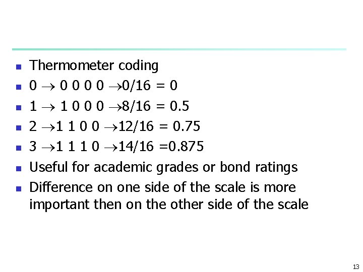
n n n n Thermometer coding 0 0 0 0/16 = 0 1 1 0 0 0 8/16 = 0. 5 2 1 1 0 0 12/16 = 0. 75 3 1 1 1 0 14/16 =0. 875 Useful for academic grades or bond ratings Difference on one side of the scale is more important then on the other side of the scale 13

Nominal Variables n n n Ex: Gender marital status, occupation 1 - treat like ordinary variables n Ex marital status 5 codes: n Single, divorced, maried, widowed, unknown n Mapped to -1, -0. 5, 0, 0. 5, 1 Network treat them ordinal Even though order does not make sence 14

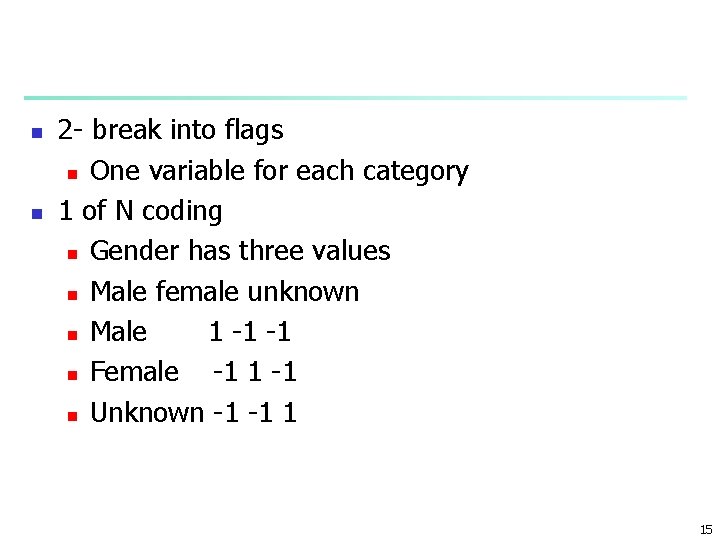
n n 2 - break into flags n One variable for each category 1 of N coding n Gender has three values n Male female unknown n Male 1 -1 -1 n Female -1 1 -1 n Unknown -1 -1 1 15

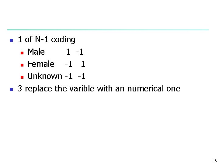
n n 1 of N-1 coding n Male 1 -1 n Female -1 1 n Unknown -1 -1 3 replace the varible with an numerical one 16

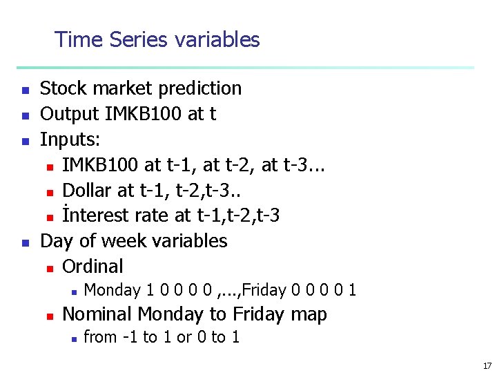
Time Series variables n n Stock market prediction Output IMKB 100 at t Inputs: n IMKB 100 at t-1, at t-2, at t-3. . . n Dollar at t-1, t-2, t-3. . n İnterest rate at t-1, t-2, t-3 Day of week variables n Ordinal n n Monday 1 0 0 , . . . , Friday 0 0 1 Nominal Monday to Friday map n from -1 to 1 or 0 to 1 17

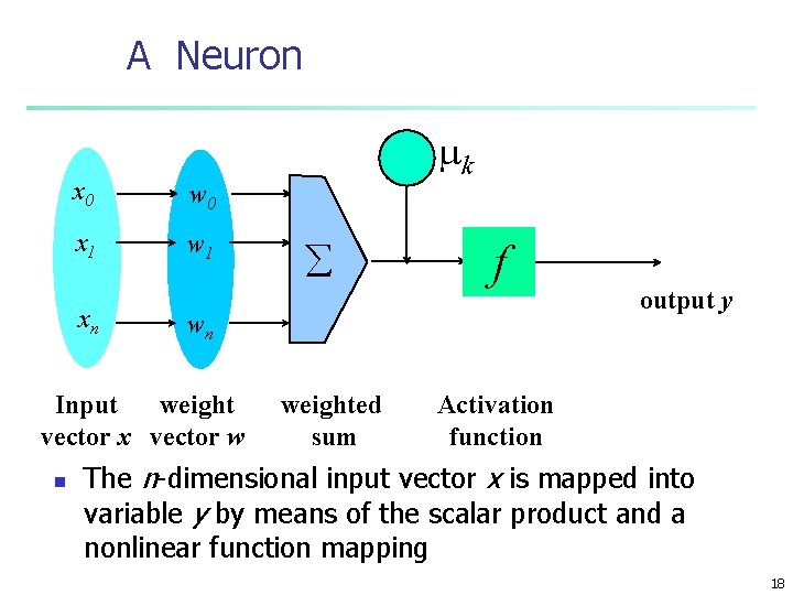
A Neuron x 0 w 0 x 1 w 1 xn å f wn Input weight vector x vector w n - mk weighted sum output y Activation function The n-dimensional input vector x is mapped into variable y by means of the scalar product and a nonlinear function mapping 18

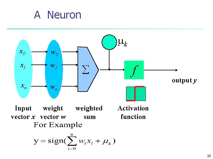
A Neuron x 0 w 0 x 1 w 1 xn - mk å f wn Input weight vector x vector w weighted sum output y Activation function 19

Network Training n n The ultimate objective of training n obtain a set of weights that makes almost all the tuples in the training data classified correctly Steps n Initialize weights with random values n repeat until classification error is lower then a threshold (epoch) n n Feed the input tuples into the network one by one For each unit n n Compute the net input to the unit as a linear combination of all the inputs to the unit Compute the output value using the activation function Compute the error Update the weights and the bias 20

Example: Stock market prediction n n input variables: n individual stock prices at t-1, t-2, t-3, . . . n stock index at t-1, t-2, t-3, n inflation rate, interest rate, exchange rates $ output variable: n predicted stock price next time train the network with known cases n adjust weights n experiment with different topologies n test the network use the tested network for predicting unknown stock prices 21

Other business Applications (1) n Marketing and sales n Prediction n n Classification n n Sales forecasting Price elasticity forecasting Customer responce Target marketing Customer satisfaction Loyalty and retention Clustering n segmentation 22

Other business Applications (1) n n n Risk Management n Credit scoring n Financial health Clasification n Bankruptcy clasification n Fraud detection n Credit scoring Clustering n Credit scoring n Risk assesment 23

Other business Applications (1) n Finance n Prediction n n Clasification n Hedging Future prediction Forex stock prediction Stock trend clasification Bond rating Clustering n n Economic rating Mutual fond selection 24

Perceptrons n n n n n WK 91 sec 4. 2 N inputs Ii i: 1. . N single output O two classes C 0 and C 1 denoted by 0 and 1 one node output: O=1 if w 1 I 1+ w 2 I 2+. . . +wn. In+w 0>0 O=0 if w 1 I 1+ w 2 I 2+. . . +wn. In+w 0<0 sometimes is used for constant term for w 0 n called bias or treshold in ANN 25

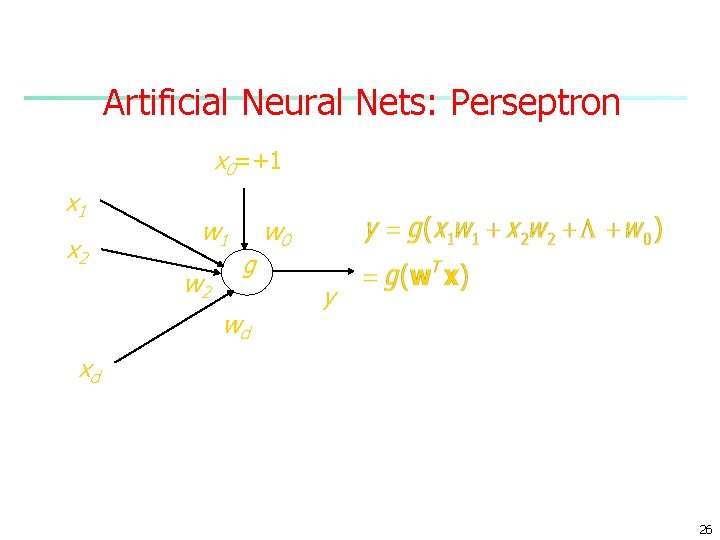
Artificial Neural Nets: Perseptron x 0=+1 x 2 w 1 w 2 g wd w 0 y xd 26

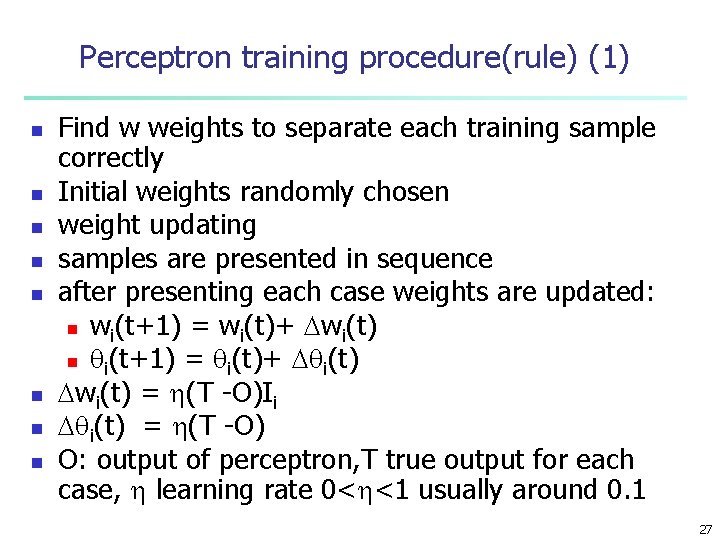
Perceptron training procedure(rule) (1) n n n n Find w weights to separate each training sample correctly Initial weights randomly chosen weight updating samples are presented in sequence after presenting each case weights are updated: n wi(t+1) = wi(t)+ wi(t) n i(t+1) = i(t)+ i(t) wi(t) = (T -O)Ii i(t) = (T -O) O: output of perceptron, T true output for each case, learning rate 0< <1 usually around 0. 1 27

Perceptron training procedure (rule) (2) n n each case is presented and weights are updated after presenting each case if n the error is not zero n then present all cases ones n each such cycle is called an epoch unit error is zero for perfectly separable samples 28

n Perceptron convergence theorem: n if the sample is linearly separable the perceptron will eventually converge: separate all the sample correctly n n error =0 the learning rate can be even one n This slows down the convergence to increase stability n it is gradually decreased linearly separable: a line or hyperplane can separate all the sample correctly 29

n n n If classes are not perfectly linearly separable if a plane or line can not separate classes completely The procedure will not converge and will keep on cycling through the data forever 30

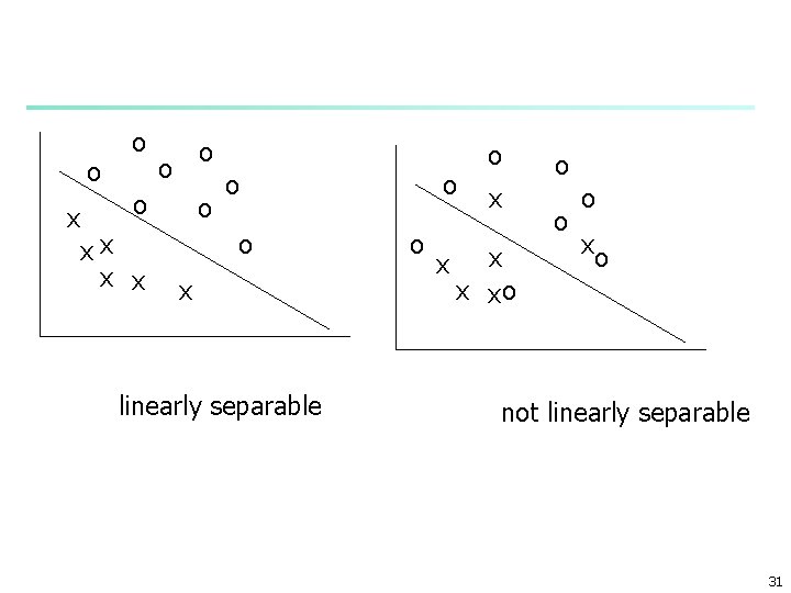
o x o o xx x x o o o x linearly separable o o o x x xo o xo not linearly separable 31

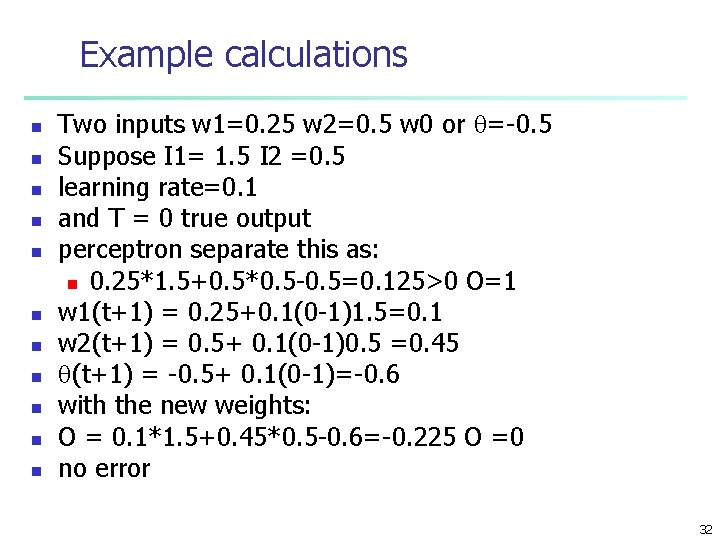
Example calculations n n n Two inputs w 1=0. 25 w 2=0. 5 w 0 or =-0. 5 Suppose I 1= 1. 5 I 2 =0. 5 learning rate=0. 1 and T = 0 true output perceptron separate this as: n 0. 25*1. 5+0. 5*0. 5 -0. 5=0. 125>0 O=1 w 1(t+1) = 0. 25+0. 1(0 -1)1. 5=0. 1 w 2(t+1) = 0. 5+ 0. 1(0 -1)0. 5 =0. 45 (t+1) = -0. 5+ 0. 1(0 -1)=-0. 6 with the new weights: O = 0. 1*1. 5+0. 45*0. 5 -0. 6=-0. 225 O =0 no error 32

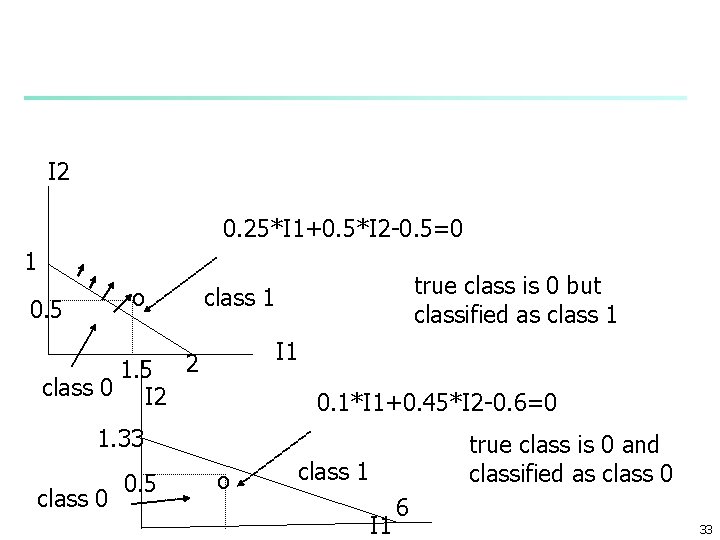
I 2 0. 25*I 1+0. 5*I 2 -0. 5=0 1 o 0. 5 1. 5 class 0 I 2 true class is 0 but classified as class 1 I 1 2 0. 1*I 1+0. 45*I 2 -0. 6=0 1. 33 class 0 0. 5 o true class is 0 and classified as class 0 class 1 I 1 6 33

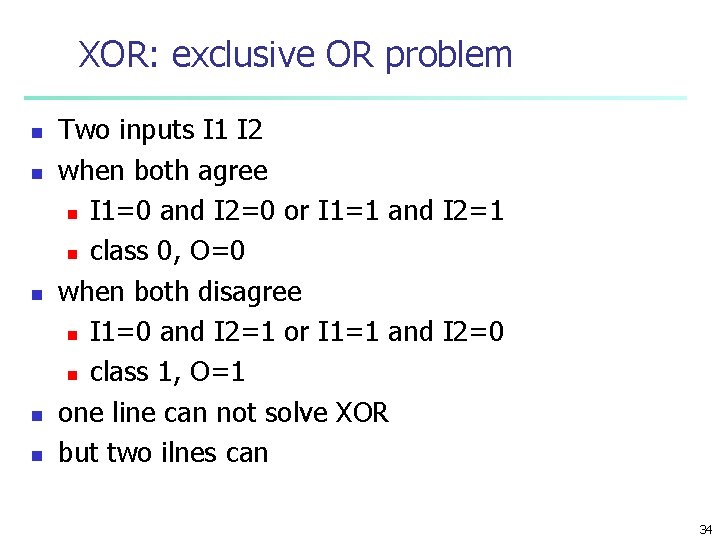
XOR: exclusive OR problem n n n Two inputs I 1 I 2 when both agree n I 1=0 and I 2=0 or I 1=1 and I 2=1 n class 0, O=0 when both disagree n I 1=0 and I 2=1 or I 1=1 and I 2=0 n class 1, O=1 one line can not solve XOR but two ilnes can 34

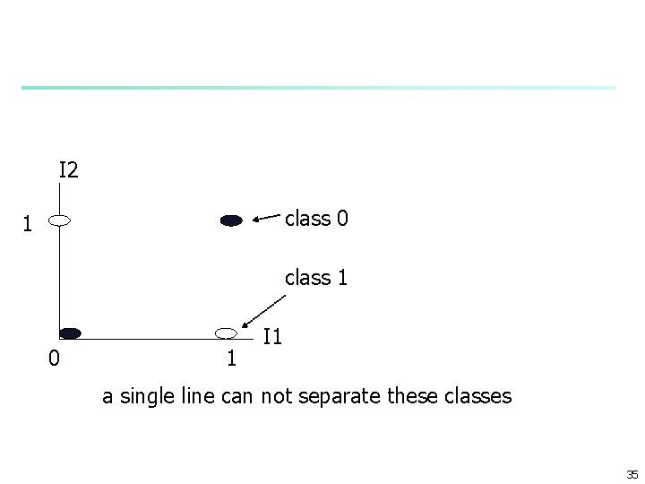
I 2 class 0 1 class 1 0 1 I 1 a single line can not separate these classes 35

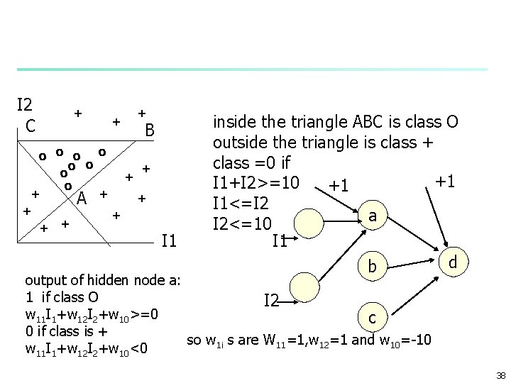
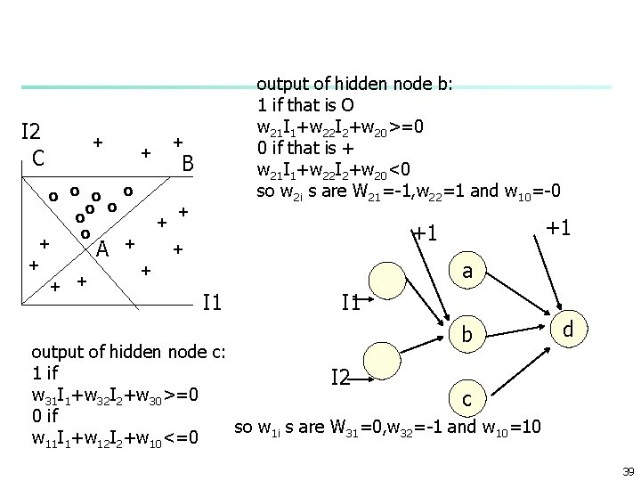
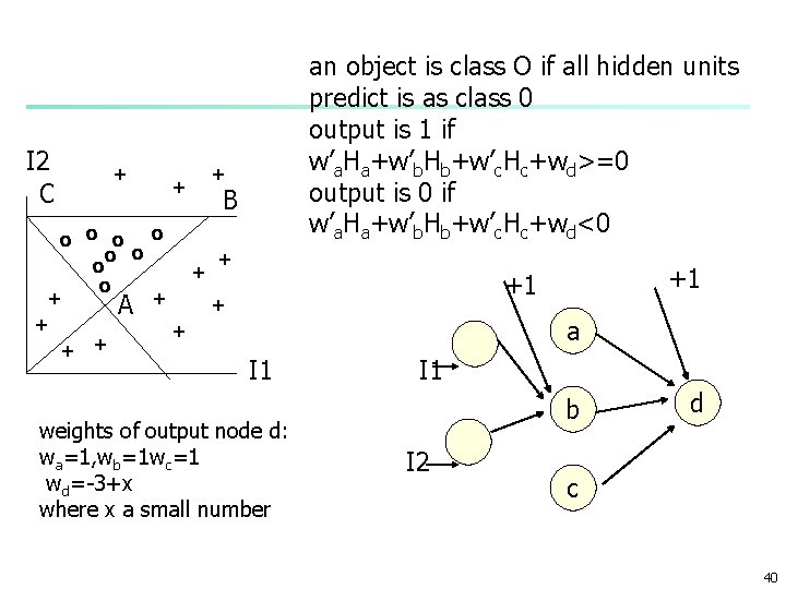
Multi-layer networks n n n Study 4. 3 In WK One layer networks can separate a hyperplane two layer networks can any convex region and three layer networks can separate any non convex boundary Examples see notes 36

ANN for classification o 2 o 1 o. K w. Kd x 0=+1 x 2 xd 37

I 2 C + + + B o o o + o + + A + + + I 1 inside the triangle ABC is class O outside the triangle is class + class =0 if +1 I 1+I 2>=10 +1 I 1<=I 2 a I 2<=10 I 1 d b output of hidden node a: 1 if class O I 2 w 11 I 1+w 12 I 2+w 10>=0 c 0 if class is + so w 1 i s are W 11=1, w 12=1 and w 10=-10 w 11 I 1+w 12 I 2+w 10<0 38

I 2 C + + output of hidden node b: 1 if that is O w 21 I 1+w 22 I 2+w 20>=0 0 if that is + w 21 I 1+w 22 I 2+w 20<0 so w 2 i s are W 21=-1, w 22=1 and w 10=-0 + B o o o + o + + A + + +1 +1 a I 1 b output of hidden node c: 1 if I 2 w 31 I 1+w 32 I 2+w 30>=0 c 0 if so w 1 i s are W 31=0, w 32=-1 and w 10=10 w 11 I 1+w 12 I 2+w 10<=0 d 39

I 2 C + + an object is class O if all hidden units predict is as class 0 output is 1 if w’a. Ha+w’b. Hb+w’c. Hc+wd>=0 output is 0 if w’a. Ha+w’b. Hb+w’c. Hc+wd<0 + B o o o + o + + A + + +1 +1 a I 1 weights of output node d: wa=1, wb=1 wc=1 wd=-3+x where x a small number I 1 b I 2 d c 40

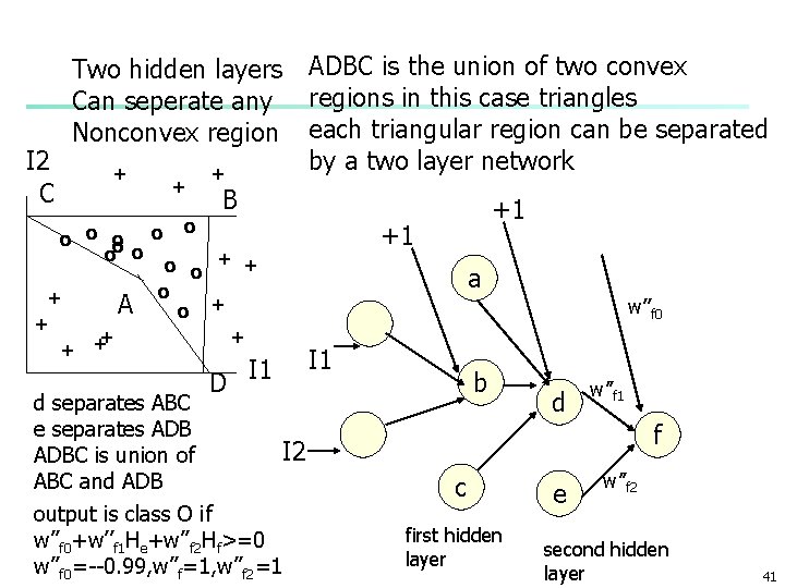
I 2 C Two hidden layers Can seperate any Nonconvex region + + o o o o + A + + o + ADBC is the union of two convex regions in this case triangles each triangular region can be separated by a two layer network B o o + + D I 1 d separates ABC e separates ADB I 2 ADBC is union of ABC and ADB output is class O if w’’f 0+w’’f 1 He+w’’f 2 Hf>=0 w’’f 0=--0. 99, w’’f=1, w’’f 2=1 +1 +1 a w’’f 0 I 1 b d w’’f 1 f c first hidden layer e w’’f 2 second hidden layer 41

n n n In practice boundaries are not known but increasing number of hidden node: two layer perceptron can separate any convex region n if it is perfectly separable adding a second hidden layer and or ing the convex regions any nonconvex boundary can be separated n if it is perfectly separable Weights are unknown but are found by training the network 42

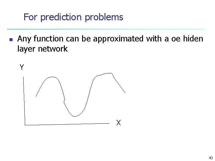
For prediction problems n Any function can be approximated with a oe hiden layer network Y X 43

Network Training n n The ultimate objective of training n obtain a set of weights that makes almost all the tuples in the training data classified correctly Steps n Initialize weights with random values n Feed the input tuples into the network one by one n For each unit n n Compute the net input to the unit as a linear combination of all the inputs to the unit Compute the output value using the activation function Compute the error Update the weights and the bias 44

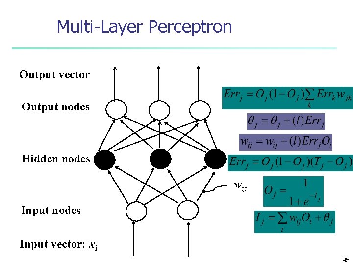
Multi-Layer Perceptron Output vector Output nodes Hidden nodes wij Input nodes Input vector: xi 45

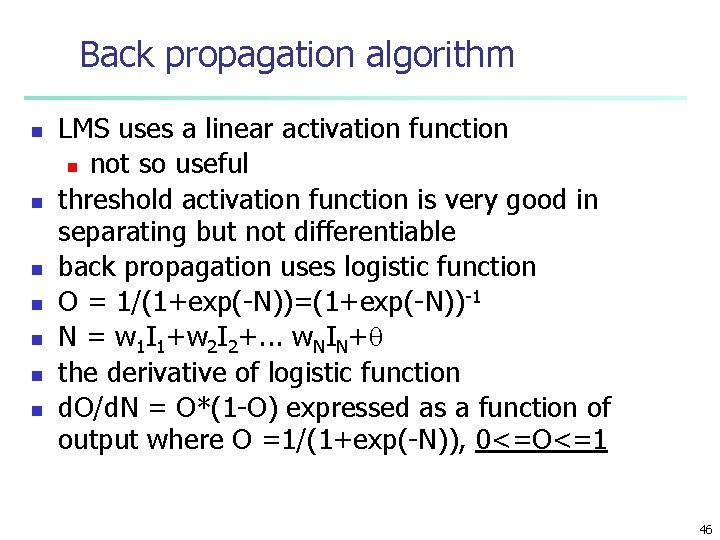
Back propagation algorithm n n n n LMS uses a linear activation function n not so useful threshold activation function is very good in separating but not differentiable back propagation uses logistic function O = 1/(1+exp(-N))=(1+exp(-N))-1 N = w 1 I 1+w 2 I 2+. . . w. NIN+ the derivative of logistic function d. O/d. N = O*(1 -O) expressed as a function of output where O =1/(1+exp(-N)), 0<=O<=1 46

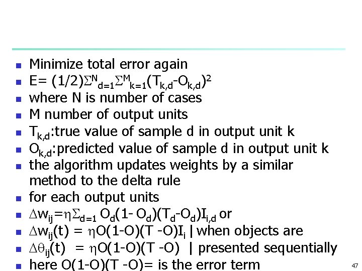
n n n Minimize total error again E= (1/2) Nd=1 Mk=1(Tk, d-Ok, d)2 where N is number of cases M number of output units Tk, d: true value of sample d in output unit k Ok, d: predicted value of sample d in output unit k the algorithm updates weights by a similar method to the delta rule for each output units wij= d=1 Od(1 - Od)(Td-Od)Ii, d or wij(t) = O(1 -O)(T -O)Ii | when objects are ij(t) = O(1 -O)(T -O) | presented sequentially here O(1 -O)(T -O)= is the error term 47

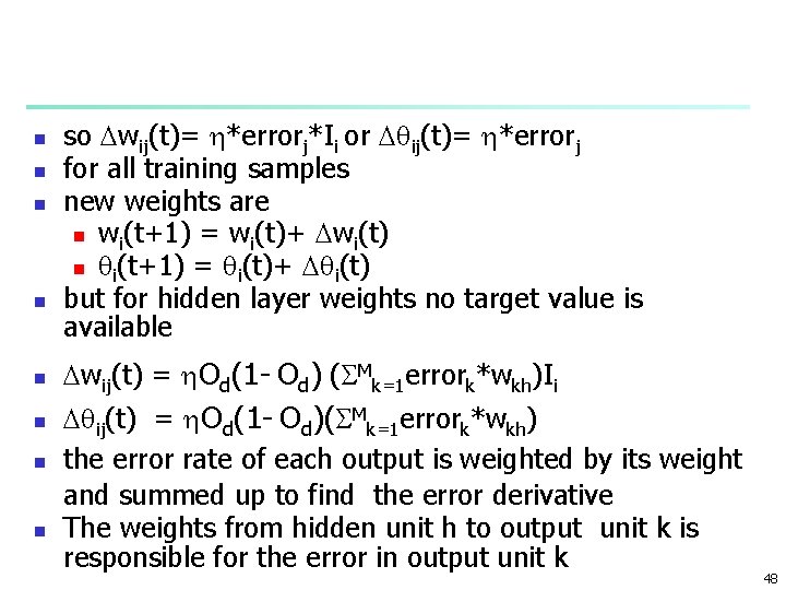
n n n n so wij(t)= *errorj*Ii or ij(t)= *errorj for all training samples new weights are n wi(t+1) = wi(t)+ wi(t) n i(t+1) = i(t)+ i(t) but for hidden layer weights no target value is available wij(t) = Od(1 - Od) ( Mk=1 errork*wkh)Ii ij(t) = Od(1 - Od)( Mk=1 errork*wkh) the error rate of each output is weighted by its weight and summed up to find the error derivative The weights from hidden unit h to output unit k is responsible for the error in output unit k 48

Example: Sample iterations n n A network suggested to solve the XOR problem figure 4. 7 of WK page 96 -99 learning rate is 1 for simplicity I 1=I 2=1 T =0 true output 49

I 1: 1 0. 1 O 3: 0. 65 0. 3 -0. 2 O 5: 0. 63 -0. 4 I 2: 1 0. 4 O 4: 0. 48 50

51

Exercise n Carry out one more iteration for the XOR problem 52

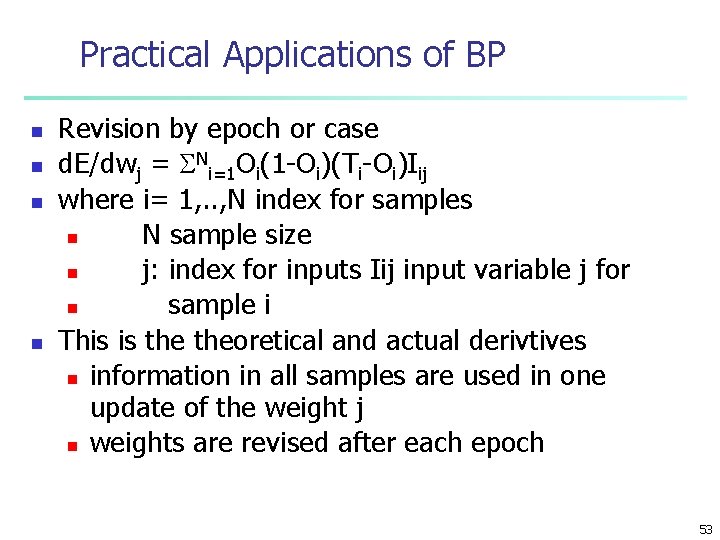
Practical Applications of BP n n Revision by epoch or case d. E/dwj = Ni=1 Oi(1 -Oi)(Ti-Oi)Iij where i= 1, . . , N index for samples n N sample size n j: index for inputs Iij input variable j for n sample i This is theoretical and actual derivtives n information in all samples are used in one update of the weight j n weights are revised after each epoch 53

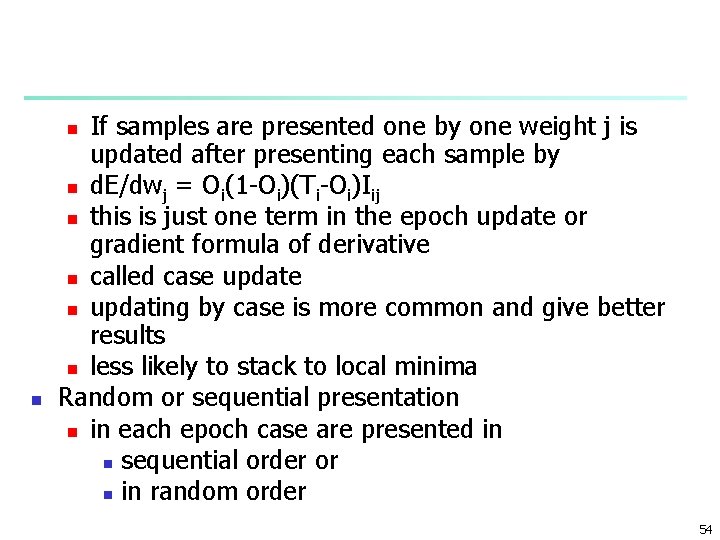
If samples are presented one by one weight j is updated after presenting each sample by n d. E/dwj = Oi(1 -Oi)(Ti-Oi)Iij n this is just one term in the epoch update or gradient formula of derivative n called case update n updating by case is more common and give better results n less likely to stack to local minima Random or sequential presentation n in each epoch case are presented in n sequential order or n in random order n n 54

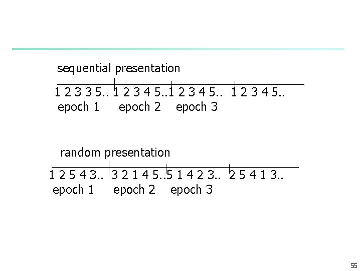
sequential presentation 1 2 3 3 5. . 1 2 3 4 5. . epoch 1 epoch 2 epoch 3 random presentation 1 2 5 4 3. . 3 2 1 4 5. . 5 1 4 2 3. . 2 5 4 1 3. . epoch 1 epoch 2 epoch 3 55

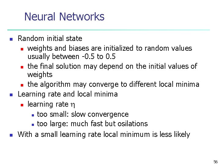
Neural Networks n n n Random initial state n weights and biases are initialized to random values usually between -0. 5 to 0. 5 n the final solution may depend on the initial values of weights n the algorithm may converge to different local minima Learning rate and local minima n learning rate n too small: slow convergence n too large: much fast but osilations With a small learning rate local minimum is less likely 56

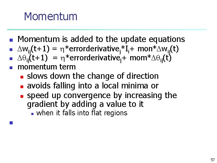
Momentum n n Momentum is added to the update equations wij(t+1) = *errorderivativej*Ii+ mon* wij(t) ij(t+1) = *errorderivativej+ mom* ij(t) momentum term n n n slows down the change of direction avoids falling into a local minima or speed up convergence by increasing the gradient by adding a value to it n when it falls into flat regions n 57

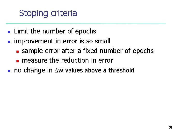
Stoping criteria n n n Limit the number of epochs improvement in error is so small n sample error after a fixed number of epochs n measure the reduction in error no change in w values above a threshold 58

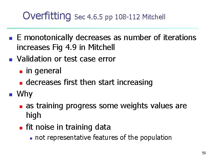
Overfitting n n n Sec 4. 6. 5 pp 108 -112 Mitchell E monotonically decreases as number of iterations increases Fig 4. 9 in Mitchell Validation or test case error n in general n decreases first then start increasing Why n as training progress some weights values are high n fit noise in training data n not representative features of the population 59

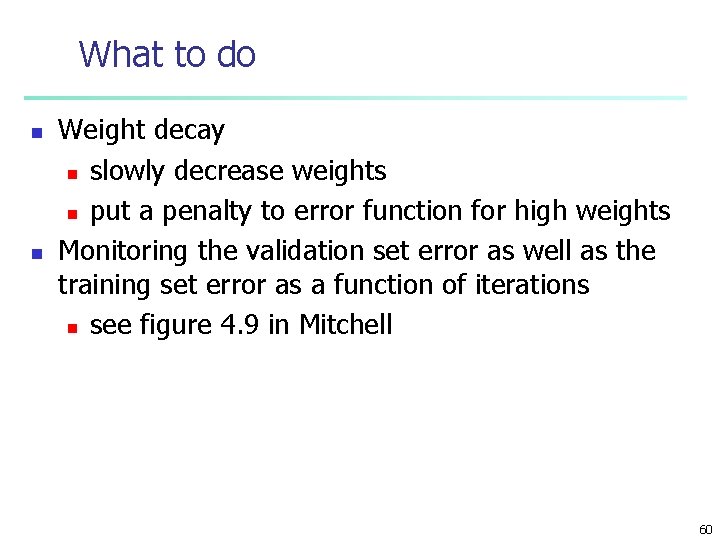
What to do n n Weight decay n slowly decrease weights n put a penalty to error function for high weights Monitoring the validation set error as well as the training set error as a function of iterations n see figure 4. 9 in Mitchell 60

Error and Complexity n n Sec 4. 4 of WK pp 102 -107 error rate on the training set decreases as number of hidden units is increased error rate on test set first decreases flatten out then start increasing as number of hidden layers is increased Start with zero hidden units n increase gradually the number of units in hidden layer n at each network size n 10 fold cross validation or n sampling the different initial weights n may be used to estimate error. n error may be averaged 61

A General Network Training Procedure n n n Define the problem Select input and output variables Make necessary transformations Decide on algorithm n gradient decent or stochastic approximation (delta rule) Choose the transfer function n logistic, hyperbolic tangent Select a learning rate a momentum n after experimenting with possibly different rates 62

A General Network Training Procedure cnt n n n Determine the stopping criteria n after error decreases by to a level or n number of epochs Start from zero hidden units increment number of hidden units n for each number of hidden units repeat n n train the network on training data set perform cross validation to estimate test error rate by averaging on different test samples n n for a set of initial weights find best initial weights 63

Neural Network Approach n n Neural network approaches n Represent each cluster as an exemplar, acting as a “prototype” of the cluster n New objects are distributed to the cluster whose exemplar is the most similar according to some distance measure Typical methods n SOM (Soft-Organizing feature Map) n Competitive learning n n Involves a hierarchical architecture of several units (neurons) Neurons compete in a “winner-takes-all” fashion for the object currently being presented 65

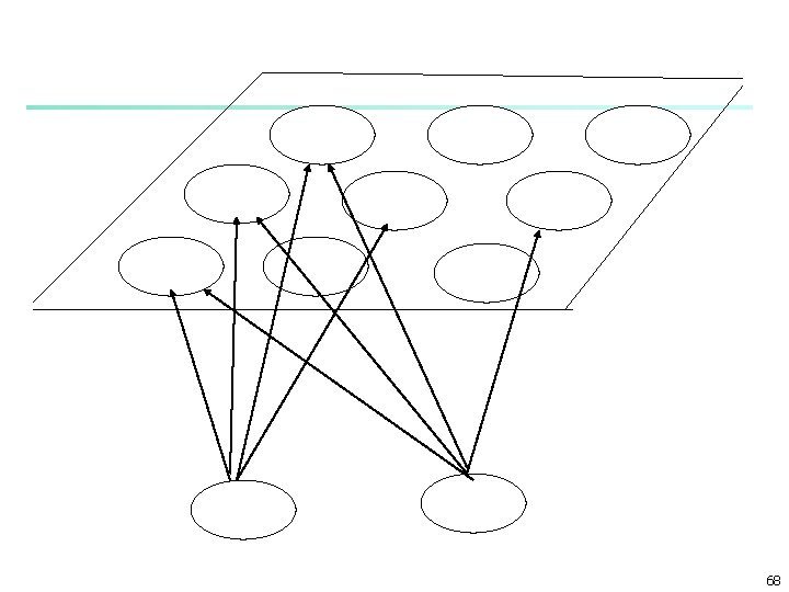
Self-Organizing Feature Map (SOM) n n SOMs, also called topological ordered maps, or Kohonen Self-Organizing Feature Map (KSOMs) It maps all the points in a high-dimensional source space into a 2 to 3 -d target space, s. t. , the distance and proximity relationship (i. e. , topology) are preserved as much as possible Similar to k-means: cluster centers tend to lie in a low-dimensional manifold in the feature space Clustering is performed by having several units competing for the current object n The unit whose weight vector is closest to the current object wins n The winner and its neighbors learn by having their weights adjusted n SOMs are believed to resemble processing that can occur in the brain n Useful for visualizing high-dimensional data in 2 - or 3 -D space 66

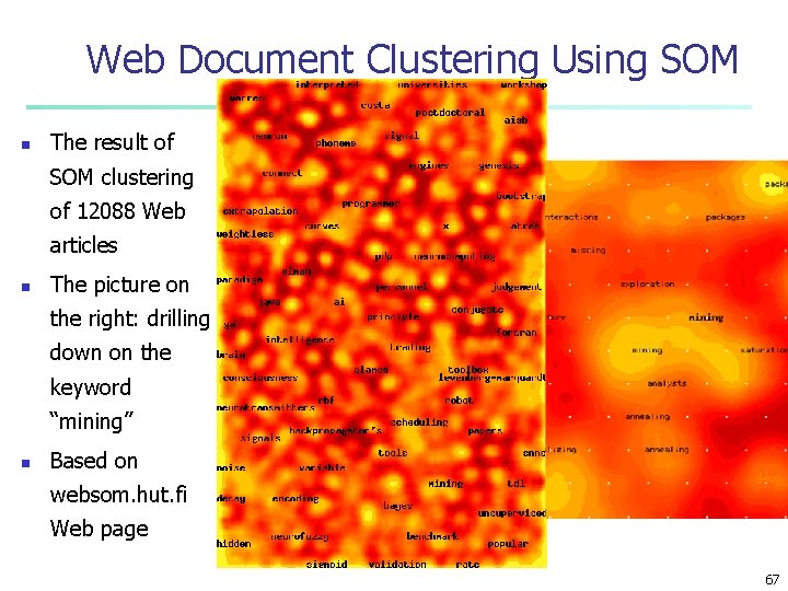
Web Document Clustering Using SOM n The result of SOM clustering of 12088 Web articles n The picture on the right: drilling down on the keyword “mining” n Based on websom. hut. fi Web page 67

68