Data Manipulation with dplyr EPID 799 C Lecture

The Tidyverse • A collection of packages for data manipulation, exploration, and visualization. •

Data Manipulation with dplyr “A grammar of data manipulation, providing a consistent set of

dplyr Key Functions • select() • filter() • arrange() • summarise() • mutate() •

dplyr Key Functions • select() • Picks variables (columns) based on their names.

dplyr Key Functions • filter() • Picks observations (rows) based on their values.

dplyr Key Functions • arrange() • Changes the ordering of the rows based on

dplyr Key Functions • summarise() • Reduces multiple values down to a single summary

dplyr Key Functions • mutate() • Adds new variables that are functions of existing

dplyr Key Functions • group_by() • Performs data operations on groups that are defined

Key Functions • select() • Picks variables (columns) based on their names • filter()

Key Operator: The Pipe %>% • Enables you to pass the object on left

Basic Structure • Use the key functions and pipe to chain together multiple simple

Basic Structure #Prints output to the console: Dataset %>% Select rows or columns to

dplyr examples with the births dataset • Based on HW #3. Feel free to

Example 1: Descriptive Statistics by Group For each value of maternal age, we are

#Getting started births %>% filter(!is. na(mage) & !is. na(pnc 5) & !is. na(preterm)) %>%

births %>% filter(!is. na(mage) & !is. na(pnc 5) & !is. na(preterm)) %>% group_by(mage) %>%

In Console: Viewing object saved in environment:

#Building on this code to get numbers of births that received early prenatal care

#Finally, use our summary variables to calculate percentages births %>% filter(!is. na(mage) & !is.

Example 1: Descriptive Statistics by Group Pseudo-code: use the births dataset, then filter out

#Our code: Filtered, grouped data %>% summarise(n=n(), pnc 5=sum(pnc 5, na. rm=T), preterm=sum(preterm, na.

Example 2: Descriptive Statistics by Group, (for many variables) • For each value of

Example 2: Descriptive Statistics by Group, (for many variables) • Instead, use “scoped variants”

births %>% select(mage, totpreg, lbliving, visits, wksgest) %>% group_by(mage) %>% summarise_all(mean, na. rm=T) #is

More on scoped variants of dplyr verb • With scoped variants of summarise or

Example 3: Introducing Joins to incorporate county-level data • For each NC county, we

#We can accomplish this with the data we have: births %>% group_by(cores) %>% summarise(pct_pnc

Example 3: Introducing Joins to incorporate county-level data • We’ll use a ‘helper’ Excel

#In keeping with a common theme, many ways to accomplish this! births_helper <- left_join(births,

births_helper %>% group_by(county_name) %>% summarise_at(c("pnc 5", "preterm"), mean, na. rm=T)

Next Steps • Lectures on 10/1, 10/3: Data visualization with ggplot • Build on

Slides: 46

Download presentation

Data Manipulation with dplyr EPID 799 C, Lecture 8 Wednesday, Sept. 26, 2018

The Tidyverse • A collection of packages for data manipulation, exploration, and visualization. • Share a common philosophy of R programming and work in harmony. • Core tidyverse packages: dplyr ggplot 2 purrr tibble tidyr readr Focus of lectures today and next week Brief intro / will continue to weave into lecture throughout semester

Data Manipulation with dplyr “A grammar of data manipulation, providing a consistent set of verbs that help you solve the most common data manipulation challenges. ” • Resources for getting started: • http: //dplyr. tidyverse. org/ • https: //cran. r-project. org/web/packages/dplyr/vignettes/dplyr. html • https: //www. rstudio. com/wp-content/uploads/2015/02/data-wranglingcheatsheet. pdf • http: //r 4 ds. had. co. nz/transform. html

dplyr Key Functions • select() • filter() • arrange() • summarise() • mutate() • group_by()

dplyr Key Functions • select() • Picks variables (columns) based on their names.

dplyr Key Functions • filter() • Picks observations (rows) based on their values.

dplyr Key Functions • arrange() • Changes the ordering of the rows based on their values.

dplyr Key Functions • summarise() • Reduces multiple values down to a single summary value.

dplyr Key Functions • mutate() • Adds new variables that are functions of existing variables.

dplyr Key Functions • group_by() • Performs data operations on groups that are defined by variables.

Key Functions • select() • Picks variables (columns) based on their names • filter() • Picks observations (rows) based on their values • arrange() • Changes the ordering of the rows • summarise() • Reduces multiple values down to a single summary value • mutate() • Adds new variables that are functions of existing variables • group_by() • Performs data operations on groups that are defined by variables

Key Operator: The Pipe %>% • Enables you to pass the object on left hand side as first argument of function on the right hand side. • Goal of making our code easier to read. x %>% f(y) #is the same as f(x, y) x %>% f(y) %>% g(z) #is the same as g(f(x, y), z)

Basic Structure • Use the key functions and pipe to chain together multiple simple steps to achieve a more complicated result. Dataset %>% Select rows or columns to manipulate %>% Arrange or group the data %>% Calculate statistics or new variables of interest

Basic Structure #Prints output to the console: Dataset %>% Select rows or columns to manipulate %>% Arrange or group the data %>% Calculate statistics or new variables #Creates a new R object: my_summary <- Dataset %>% Select rows or columns to manipulate %>% Arrange or group the data %>% Calculate statistics or new variables

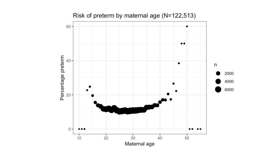
dplyr examples with the births dataset • Based on HW #3. Feel free to use or adapt this code. • NOTE: For the purposes of these examples, I am using the full births dataset (N=122, 513). In HW #3, you will use the final analytic dataset after applying all inclusion criteria (n=62, 370).

Example 1: Descriptive Statistics by Group For each value of maternal age, we are interested in: • Number of births overall • Number and percentage of births that received early prenatal care • Number and percentage of births that were preterm Among births with non-missing maternal age, prenatal care, and preterm. Pseudo-code: use the births dataset, then filter out births with missing values, then group births by mage, then summarize numbers of births, then calculate percentages for early care and preterm

#Getting started births %>% filter(!is. na(mage) & !is. na(pnc 5) & !is. na(preterm)) %>% group_by(mage) %>% summarise(n())

births %>% filter(!is. na(mage) & !is. na(pnc 5) & !is. na(preterm)) %>% group_by(mage) %>% summarise(n()) #is equivalent to births %>% filter(!is. na(mage) & !is. na(pnc 5) & !is. na(preterm)) %>% group_by(mage) %>% tally() #or count() #convenient wrappers for summarise(n())

births %>% filter(!is. na(mage) & !is. na(pnc 5) & !is. na(preterm)) %>% group_by(mage) %>% summarise(n = n()) #new columns can be named ? dplyr: : summarise

In Console: Viewing object saved in environment:

#Building on this code to get numbers of births that received early prenatal care and that were preterm (by maternal age) births %>% filter(!is. na(mage) & !is. na(pnc 5) & !is. na(preterm)) %>% group_by(mage) %>% summarise(n = n(), pnc 5 = sum(pnc 5, na. rm=T), preterm = sum(preterm, na. rm=T))

#Finally, use our summary variables to calculate percentages births %>% filter(!is. na(mage) & !is. na(pnc 5) & !is. na(preterm)) %>% group_by(mage) %>% summarise(n = n(), pnc 5 = sum(pnc 5, na. rm=T), preterm = sum(preterm, na. rm=T)) %>% mutate(perc_pnc 5 = pnc 5/n*100, perc_preterm = preterm/n*100)

Example 1: Descriptive Statistics by Group Pseudo-code: use the births dataset, then filter out births with missing values, then group births by mage, then summarize numbers of births, then calculate percentages for early care and preterm Real code: births %>% filter(!is. na(mage) & !is. na(pnc 5) & !is. na(preterm)) %>% group_by(mage) %>% summarise(n=n(), pnc 5=sum(pnc 5, na. rm=T), preterm=sum(preterm, na. rm=T) %>% mutate(perc_pnc 5 = pnc 5/n*100, perc_preterm = preterm/n*100)

#Our code: Filtered, grouped data %>% summarise(n=n(), pnc 5=sum(pnc 5, na. rm=T), preterm=sum(preterm, na. rm=T) %>% mutate(perc_pnc 5 = pnc 5/n*100, perc_preterm = preterm/n*100) #equivalently, we could have gotten the percentages using only summarise(): Filtered, grouped data %>% summarise(pct_pnc 5 = sum(pnc 5, na. rm=T)/n()*100, pct_preterm = sum(preterm, na. rm=T)/n()*100) Filtered, grouped data %>% summarise(pct_pnc 5 = mean(pnc 5, na. rm=T)*100, pct_preterm = mean(preterm, na. rm=T)*100)

Example 2: Descriptive Statistics by Group, (for many variables) • For each value of maternal age, we are interested in the mean: • • Number of pregnancies including this one (totpreg) Previous live births now living (lbliving) Number of prenatal care visits (visits) Calculated estimate of gestation (wksgest) • This is tedious: summarise(mean_totpreg = mean(totpreg, na. rm = T), mean_lbliving = mean(lbliving, na. rm = T), mean_visits = mean(visits, na. rm = T), mean_wksgest = mean(wksgest, na. rm = T))

Example 2: Descriptive Statistics by Group, (for many variables) • Instead, use “scoped variants” of summarise and mutate to apply operations on a selection of variables. summarise_all() summarise_at() summarise_if() mutate_all() mutate_at() mutate_if()

births %>% select(mage, totpreg, lbliving, visits, wksgest) %>% group_by(mage) %>% summarise_all(mean, na. rm=T) #is equivalent to: births %>% group_by(mage) %>% summarise_at(c("totpreg", "lbliving", "visits", "wksgest"), mean, na. rm=T) # but what happens here? births %>% group_by(mage) %>% summarise_if(is. numeric, mean, na. rm=T)

More on scoped variants of dplyr verb • With scoped variants of summarise or mutate, you can perform multiple functions on each column, e. g. : births %>% select(mage, totpreg, lbliving, visits, wksgest) %>% summarise_all(funs(min, median, max), na. rm=T) • There also scoped variants of filter, group_by, select, arrange… • Same three kinds of scoped variants: _all(), _at(), _if() • I’m just scratching the surface! More here: • https: //dplyr. tidyverse. org/reference/scoped. html • https: //dplyr. tidyverse. org/reference/summarise_all. html

Example 3: Introducing Joins to incorporate county-level data • For each NC county, we are interested in the percentage of births that received early prenatal care and the percentage of births that were preterm. • In our data, the variable ‘cores’ is the mother’s county of residence, coded as numbers 1 -199 with 999 for out of state.

#We can accomplish this with the data we have: births %>% group_by(cores) %>% summarise(pct_pnc 5 = mean(pnc 5, na. rm = T)*100, pct_preterm = mean(preterm, na. rm = T)*100) #But it would be helpful to have the county names…

Example 3: Introducing Joins to incorporate county-level data • We’ll use a ‘helper’ Excel spreadsheet to merge in the county names (so you don’t have to type them!). • Introducing the dplyr verbs for joining: inner_join() left_join() right_join() full_join() Mutating joins semi_join() anti_join() Filtering joins AWESOME (animated!) resource from Nick: https: //github. com/gadenbuie/tidy-animated-verbs#readme

Our two dataframes to be merged:

#In keeping with a common theme, many ways to accomplish this! births_helper <- left_join(births, helper, by = "cores") #All rows from x, and all columns from x and y

#In keeping with a common theme, many ways to accomplish this! births_helper <- left_join(births, helper, by = "cores") #All rows from x, and all columns from x and y births_helper <- right_join(helper, births, by = "cores") #All rows from y, and all columns from x and y

#In keeping with a common theme, many ways to accomplish this! births_helper <- left_join(births, helper) #All rows from x, and all columns from x and y births_helper <- right_join(helper, births) #All rows from y, and all columns from x and y It’s good to be explicit, but specifying the by-variable is not necessary here.

#In keeping with a common theme, many ways to accomplish this! births_helper <- left_join(births, helper) #All rows from x, and all columns from x and y births_helper <- right_join(helper, births) #All rows from y, and all columns from x and y births_helper <- full_join(births, helper) #All rows and all columns from both x and y

births_helper %>% group_by(county_name) %>% summarise_at(c("pnc 5", "preterm"), mean, na. rm=T)

Next Steps • Lectures on 10/1, 10/3: Data visualization with ggplot • Build on our skills for manipulating and summarizing data with dplyr • Looking ahead, we can pipe our dplyr summary data into ggplot to graph.