Data Intensive and Cloud Computing Matrices and Arrays

Data Intensive and Cloud Computing Matrices and Arrays Lecture 9

Matrices and Arrays in Python: Num. Py • We’ve already seen lists – single-dimensional data with a single type • More generically, we may want to have matrices (as in Page. Rank) or multidimensional arrays • This leads to numpy – support for numeric operations in Python • A building block for Pandas • And for Sci. Py, which is scientific programming support 2

What Do We Use Matrices / Multi. Dimensional Arrays for? • Graph adjacency matrices, and variants thereof • Rows of readings of sets of numeric values (e. g. , a suite of sensors) • Machine learning features (later in the semester!) • Images, volumes, numeric state values in a multidimensional space 3

5 Important Concepts from Linear Algebra Help! My matrix is too big to analyze by inspection. I should compute: • Frobenius Norm • Rank • Determinant • Singular Vectors / Singular Values • Eigenvectors / Eigenvalues 4

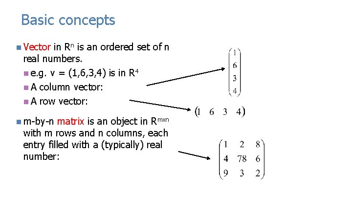
Basic concepts n Vector in Rn is an ordered set of n real numbers. n e. g. v = (1, 6, 3, 4) is in R 4 n A column vector: n A row vector: n m-by-n matrix is an object in Rmxn with m rows and n columns, each entry filled with a (typically) real number:

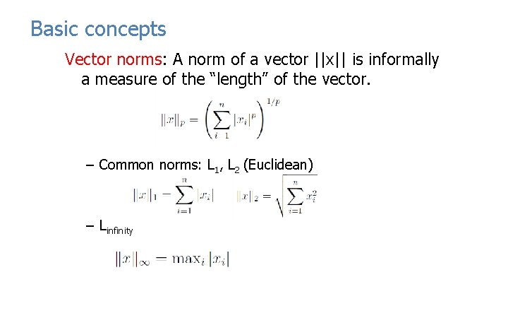
Basic concepts Vector norms: A norm of a vector ||x|| is informally a measure of the “length” of the vector. – Common norms: L 1, L 2 (Euclidean) – Linfinity

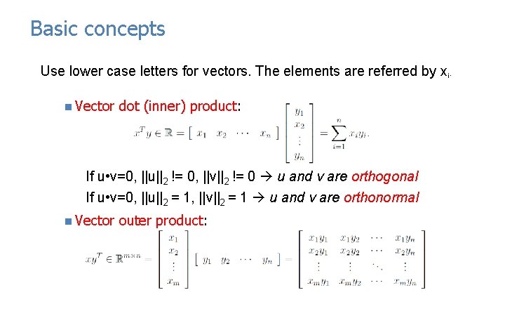
Basic concepts Use lower case letters for vectors. The elements are referred by xi. n Vector dot (inner) product: If u • v=0, ||u||2 != 0, ||v||2 != 0 u and v are orthogonal If u • v=0, ||u||2 = 1, ||v||2 = 1 u and v are orthonormal n Vector outer product:

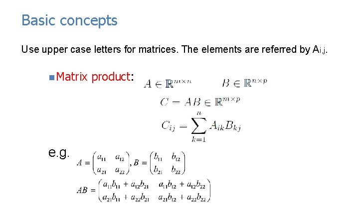
Basic concepts Use upper case letters for matrices. The elements are referred by Ai, j. n Matrix e. g. product:

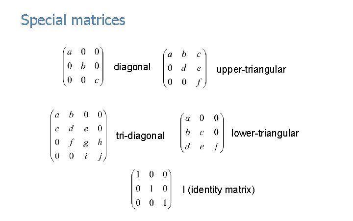
Special matrices diagonal tri-diagonal upper-triangular lower-triangular I (identity matrix)

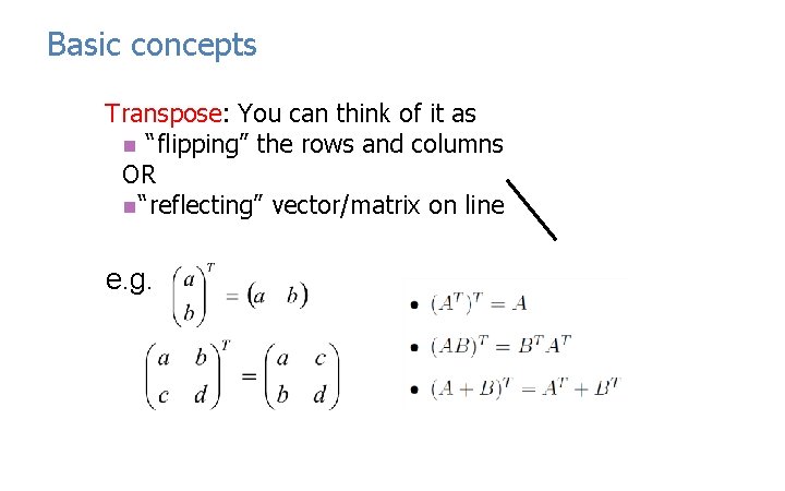
Basic concepts Transpose: You can think of it as n “flipping” the rows and columns OR n “reflecting” vector/matrix on line e. g.

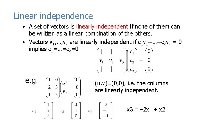
Linear independence • A set of vectors is linearly independent if none of them can be written as a linear combination of the others. • Vectors v 1, …, vk are linearly independent if c 1 v 1+…+ckvk = 0 implies c 1=…=ck=0 e. g. (u, v)=(0, 0), i. e. the columns are linearly independent. x 3 = − 2 x 1 + x 2

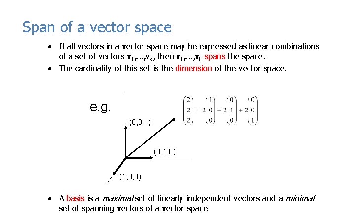
Span of a vector space • If all vectors in a vector space may be expressed as linear combinations of a set of vectors v 1, …, vk, then v 1, …, vk spans the space. • The cardinality of this set is the dimension of the vector space. e. g. (0, 0, 1) (0, 1, 0) (1, 0, 0) • A basis is a maximal set of linearly independent vectors and a minimal set of spanning vectors of a vector space

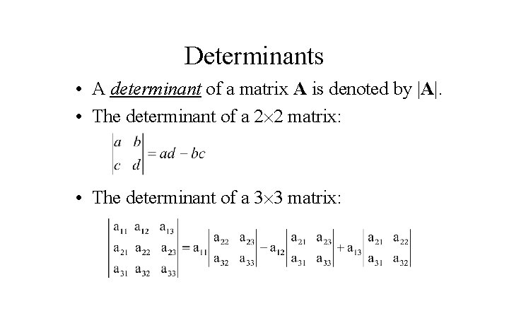
Determinants • A determinant of a matrix A is denoted by |A|. • The determinant of a 2 2 matrix: • The determinant of a 3 3 matrix:

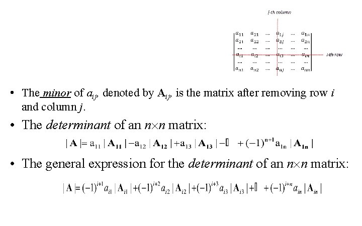
• The minor of aij, denoted by Aij, is the matrix after removing row i and column j. • The determinant of an n n matrix: • The general expression for the determinant of an n n matrix:

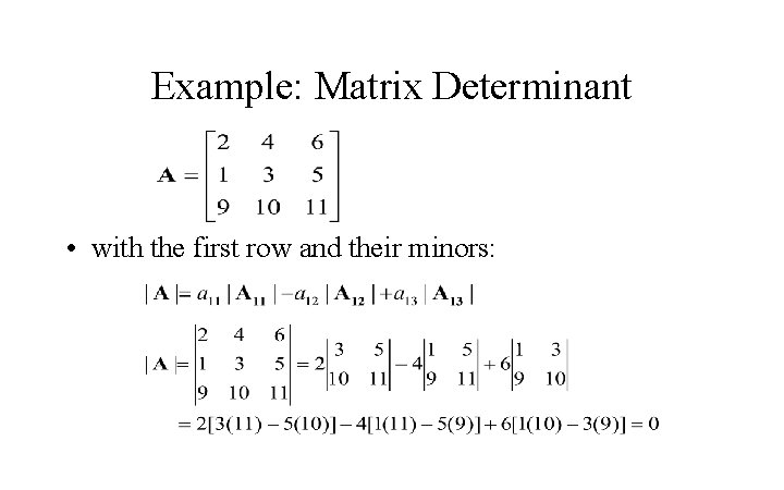
Example: Matrix Determinant • with the first row and their minors:

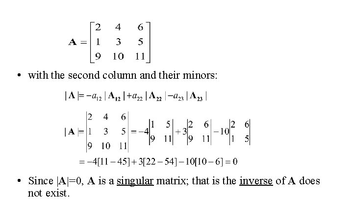
• with the second column and their minors: • Since |A|=0, A is a singular matrix; that is the inverse of A does not exist.

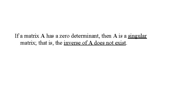
If a matrix A has a zero determinant, then A is a singular matrix; that is, the inverse of A does not exist.

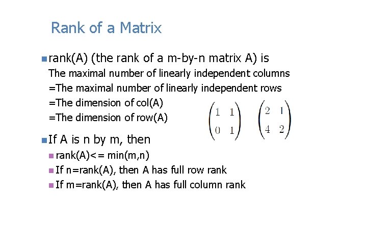
Rank of a Matrix n rank(A) (the rank of a m-by-n matrix A) is The maximal number of linearly independent columns =The maximal number of linearly independent rows =The dimension of col(A) =The dimension of row(A) n If A is n by m, then n rank(A)<= min(m, n) n If n=rank(A), then A has full row rank n If m=rank(A), then A has full column rank

Rank– Many Equivalent Definitions A matrix of r rows and c columns is said to be of order r by c. If it is a square matrix, r by r, then the matrix is of order r. The rank of a matrix equals the order of highest-order nonsingular submatrix.

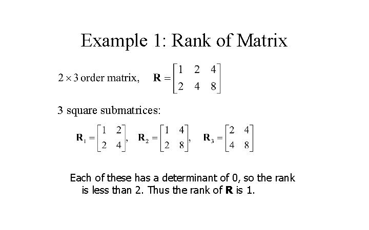
Example 1: Rank of Matrix 3 square submatrices: Each of these has a determinant of 0, so the rank is less than 2. Thus the rank of R is 1.

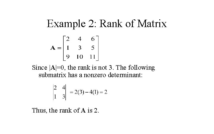
Example 2: Rank of Matrix Since |A|=0, the rank is not 3. The following submatrix has a nonzero determinant: Thus, the rank of A is 2.

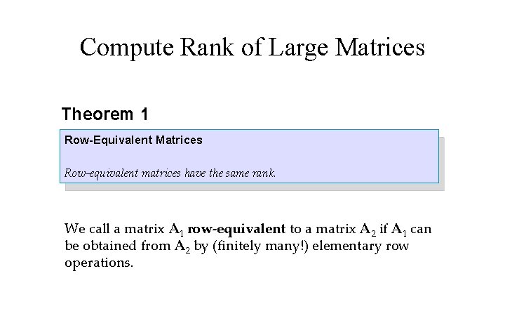
Compute Rank of Large Matrices Theorem 1 Row-Equivalent Matrices Row-equivalent matrices have the same rank. We call a matrix A 1 row-equivalent to a matrix A 2 if A 1 can be obtained from A 2 by (finitely many!) elementary row operations.

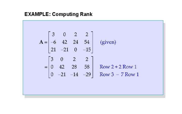
EXAMPLE: Computing Rank

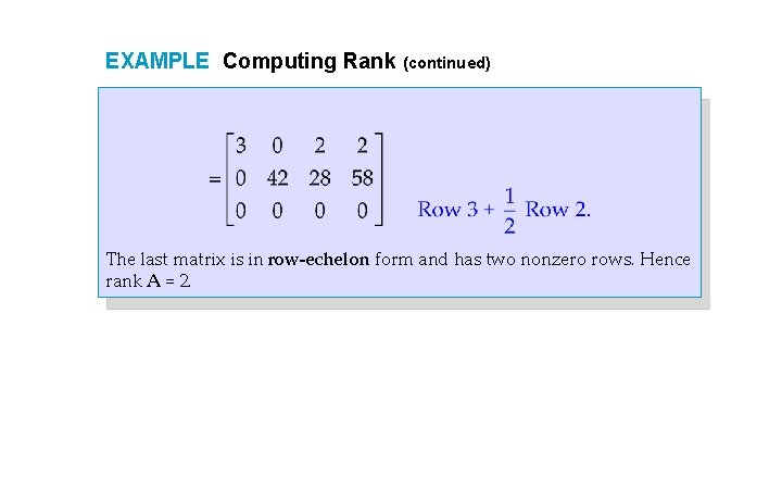
EXAMPLE Computing Rank (continued) The last matrix is in row-echelon form and has two nonzero rows. Hence rank A = 2.

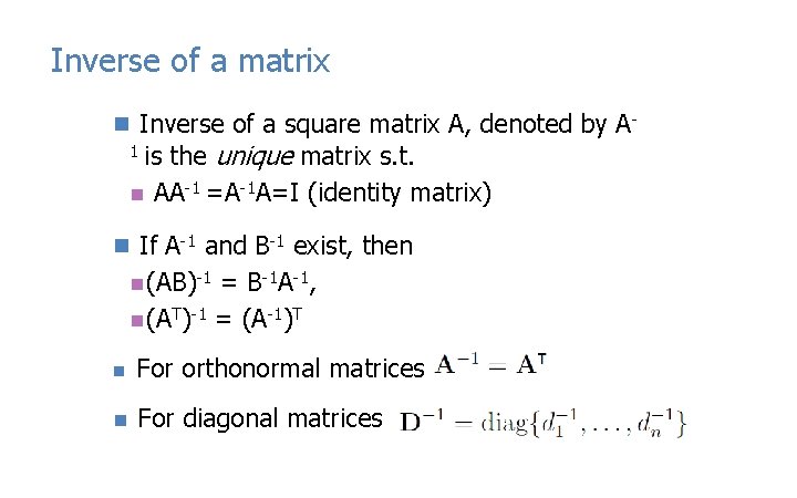
Inverse of a matrix n Inverse of a square matrix A, denoted by A- is the unique matrix s. t. n AA-1 =A-1 A=I (identity matrix) 1 n If A-1 and B-1 exist, then n (AB)-1 = B-1 A-1, n (AT)-1 = (A-1)T n For orthonormal matrices n For diagonal matrices

Python Support for Matrices

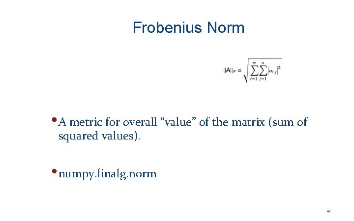
Frobenius Norm • A metric for overall “value” of the matrix (sum of squared values). • numpy. linalg. norm 27

Rank • The number of nonzero rows after a row reduction. • Yet another definition • numpy. linalg. matrix_rank 28

Determinant • A metric describing the overall “scaling factor” of the matrix. How much would multiplying by this matrix stretch the unit box? • numpy. linalg. det 29

Singular vectors / Singular Values • Start with the vector that gets stretched most by this matrix (and how much). Then, find independent others in descending order. • numpy. linalg. svd 30

Eigenvectors / Eigenvalues • The special vectors that this matrix can only scale (and by how much). • numpy. linalg. eig 31

Num. Py - Details 32

What is Num. Py? • Num. Py is the fundamental package needed for scientific computing with Python. It contains: • a powerful N-dimensional array object • basic linear algebra functions • basic Fourier transforms • sophisticated random number capabilities • tools for integrating Fortran code • tools for integrating C/C++ code 33

Num. Py documentation • Official documentation • http: //docs. scipy. org/doc/ • The Num. Py book • http: //www. tramy. us/numpybook. pdf • Example list • http: //www. scipy. org/Numpy_Example_List_With_Doc 34

The ndarray data structure • Num. Py adds a new data structure to Python – the ndarray • An N-dimensional array is a homogeneous collection of “items” indexed using N integers • Defined by: 1. 2. the shape of the array, and the kind of item the array is composed of 35

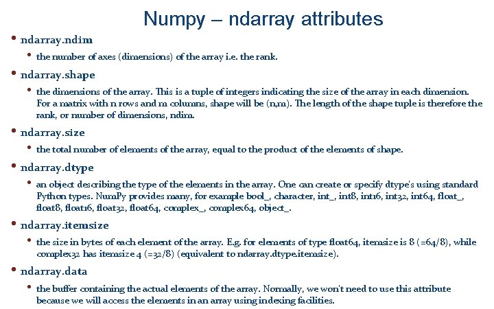
• ndarray. ndim • Numpy – ndarray attributes the number of axes (dimensions) of the array i. e. the rank. • ndarray. shape • the dimensions of the array. This is a tuple of integers indicating the size of the array in each dimension. For a matrix with n rows and m columns, shape will be (n, m). The length of the shape tuple is therefore the rank, or number of dimensions, ndim. • ndarray. size • the total number of elements of the array, equal to the product of the elements of shape. • ndarray. dtype • an object describing the type of the elements in the array. One can create or specify dtype's using standard Python types. Num. Py provides many, for example bool_, character, int_, int 8, int 16, int 32, int 64, float_, float 8, float 16, float 32, float 64, complex_, complex 64, object_. • ndarray. itemsize • the size in bytes of each element of the array. E. g. for elements of type float 64, itemsize is 8 (=64/8), while complex 32 has itemsize 4 (=32/8) (equivalent to ndarray. dtype. itemsize). • ndarray. data • the buffer containing the actual elements of the array. Normally, we won't need to use this attribute because we will access the elements in an array using indexing facilities.

Array shape • ndarrays are rectangular • The shape of the array is a tuple of N integers (one for each dimension) 37

Array item types • Every ndarray is a homogeneous collection of exactly the same data-type • every item takes up the same size block of memory • each block of memory in the array is interpreted in exactly the same way 38

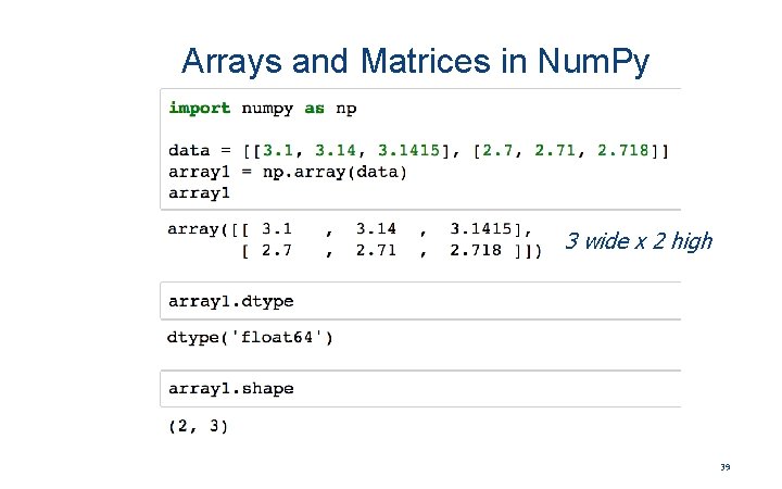
Arrays and Matrices in Num. Py 3 wide x 2 high 39

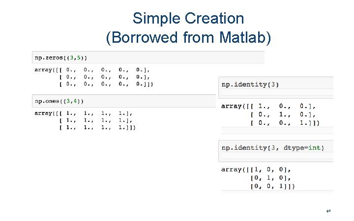
Simple Creation (Borrowed from Matlab) 40

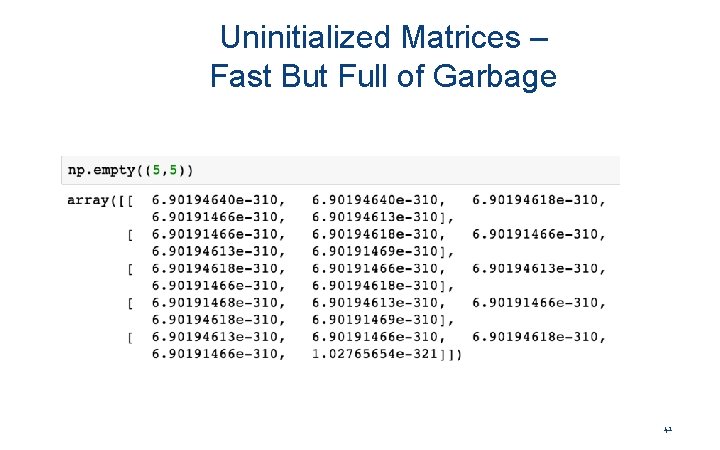
Uninitialized Matrices – Fast But Full of Garbage 41

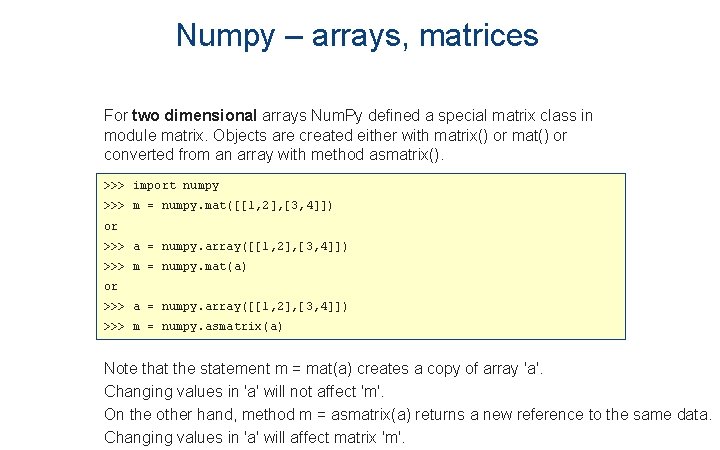
Numpy – arrays, matrices For two dimensional arrays Num. Py defined a special matrix class in module matrix. Objects are created either with matrix() or mat() or converted from an array with method asmatrix(). >>> import numpy >>> m = numpy. mat([[1, 2], [3, 4]]) or >>> a = numpy. array([[1, 2], [3, 4]]) >>> m = numpy. mat(a) or >>> a = numpy. array([[1, 2], [3, 4]]) >>> m = numpy. asmatrix(a) Note that the statement m = mat(a) creates a copy of array 'a'. Changing values in 'a' will not affect 'm'. On the other hand, method m = asmatrix(a) returns a new reference to the same data. Changing values in 'a' will affect matrix 'm'.

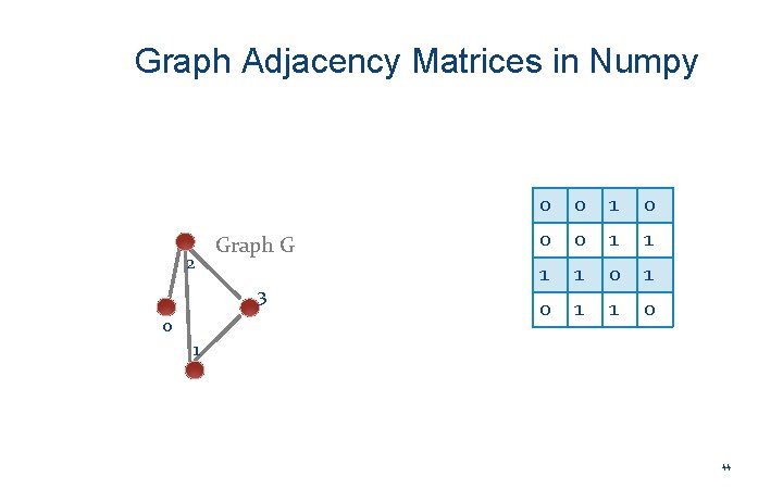
An Example of Using a Graph Adjacency Matrix 43

Graph Adjacency Matrices in Numpy 2 Graph G 3 0 0 0 1 1 1 1 0 1 44

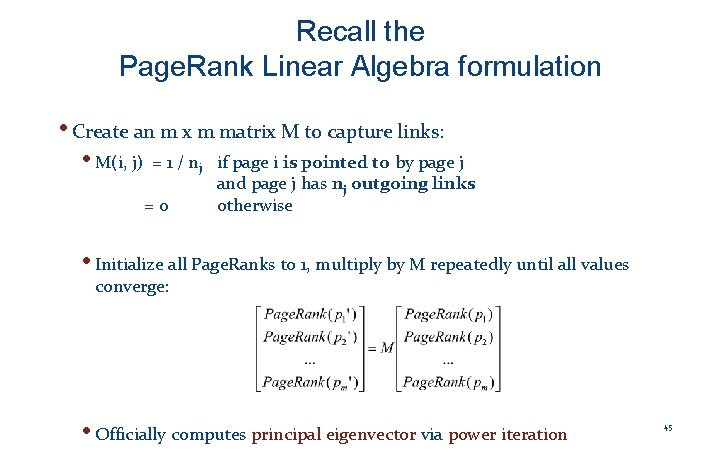
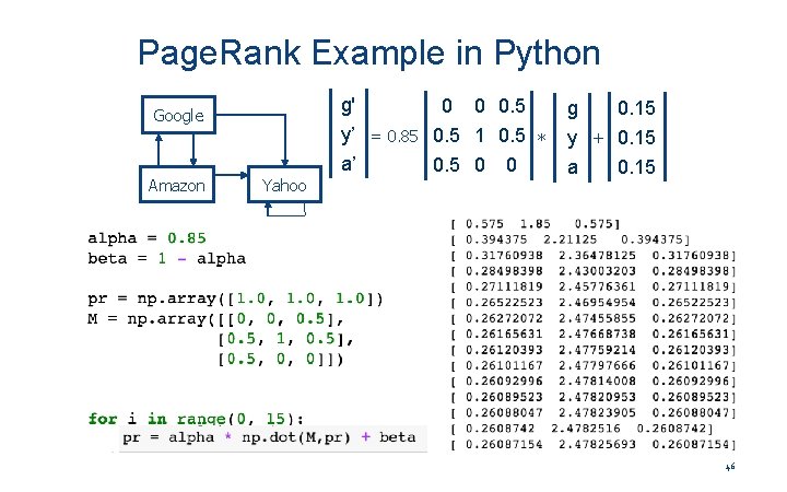
Recall the Page. Rank Linear Algebra formulation • Create an m x m matrix M to capture links: • M(i, j) = 1 / nj if page i is pointed to by page j and page j has nj outgoing links =0 otherwise • Initialize all Page. Ranks to 1, multiply by M repeatedly until all values converge: • Officially computes principal eigenvector via power iteration 45

Page. Rank Example in Python Google Amazon Yahoo g' 0 0 0. 5 y’ = 0. 85 0. 5 1 0. 5 * a’ 0. 5 0 0 0. 15 g y + 0. 15 a 46

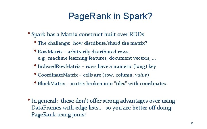
Page. Rank in Spark? • Spark has a Matrix construct built over RDDs • The challenge: how distribute/shard the matrix? • Row. Matrix – arbitrarily distributed rows. e. g. , machine learning features, document vectors, … • Indexed. Row. Matrix – rows have a numeric (long) key • Coordinate. Matrix – cells are (row, column, value) • Block. Matrix – matrix broken into “tiles” with coordinates • In general: these don’t offer strong advantages over using Data. Frames with edge lists. . . so you are better off doing Page. Rank using joins! 47

A Sketch of Page. Rank with Joins • Given dataframe edge(from, to) • Compute a dataframe transfer_weight(node, node ratio) for each • Initialize pagerank(node, score) for each node • for n iterations: • Compute weight_from_edge(from, to, weight) for each node, given existing pagerank(from, score) and transfer_weight(from, ratio) • Sum up weight_from_edge(from, to, weight) for each to – this is the new Page. Rank for the next iteration 48

Broader Matrix Manipulation University of Pennsylvania 49

Matrices Have “Bulk Operations” too • Addition and multiplication with scalars • Simple arithmetic over arrays / matrices (add, multiply) • Linear algebra operations – multiply, transpose, … • “Slicing” • Many of these are key building blocks for scientific computing 50

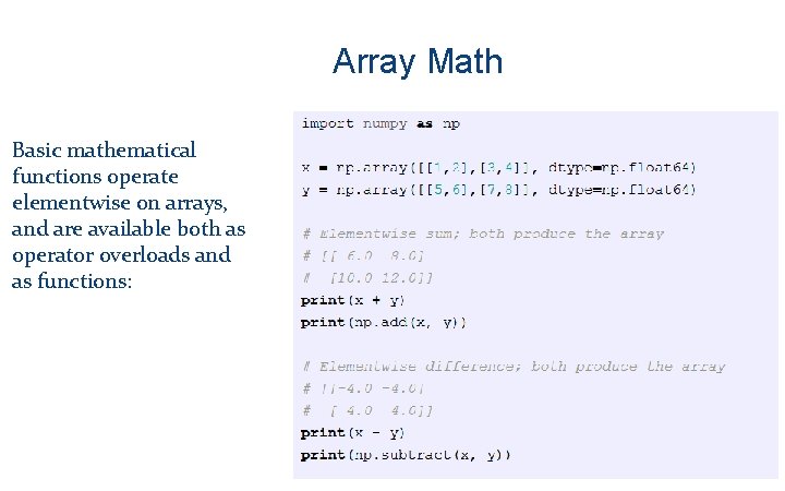
Array Math Basic mathematical functions operate elementwise on arrays, and are available both as operator overloads and as functions: 51

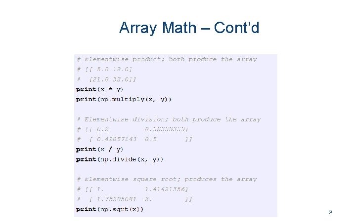
Array Math – Cont’d 52

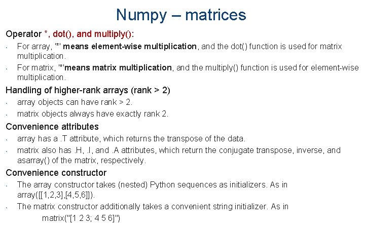
Numpy – matrices Operator *, dot(), and multiply(): • • For array, '*' means element-wise multiplication, and the dot() function is used for matrix multiplication. For matrix, '*'means matrix multiplication, and the multiply() function is used for element-wise multiplication. Handling of higher-rank arrays (rank > 2) • • array objects can have rank > 2. matrix objects always have exactly rank 2. Convenience attributes • • array has a. T attribute, which returns the transpose of the data. matrix also has. H, . I, and. A attributes, which return the conjugate transpose, inverse, and asarray() of the matrix, respectively. Convenience constructor • • The array constructor takes (nested) Python sequences as initializers. As in array([[1, 2, 3], [4, 5, 6]]). The matrix constructor additionally takes a convenient string initializer. As in matrix("[1 2 3; 4 5 6]")

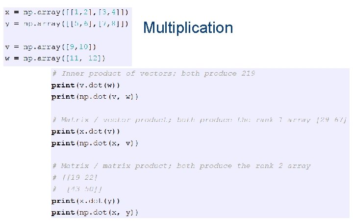
Multiplication 54

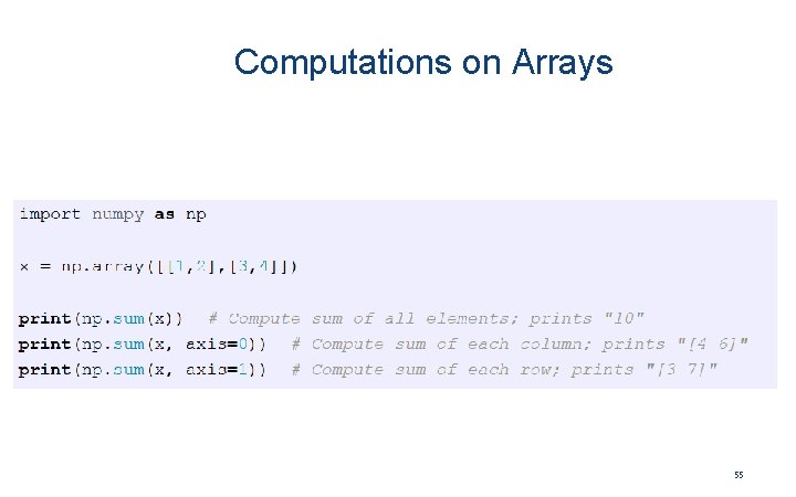
Computations on Arrays 55

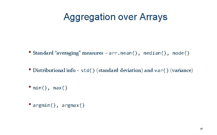
Aggregation over Arrays • Standard “averaging” measures – arr. mean(), median(), mode() • Distributional info – std() (standard deviation) and var() (variance) • min(), max() • argmin(), argmax() 56

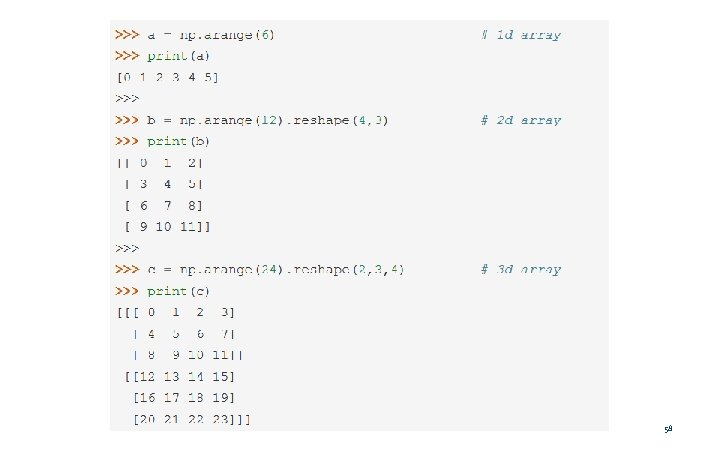
Printing Arrays When you print an array, Num. Py displays it in a similar way to nested lists, but with the following layout: • the last axis is printed from left to right, • the second-to-last is printed from top to bottom, • the rest are also printed from top to bottom, with each slice separated from the next by an empty line. 57

58

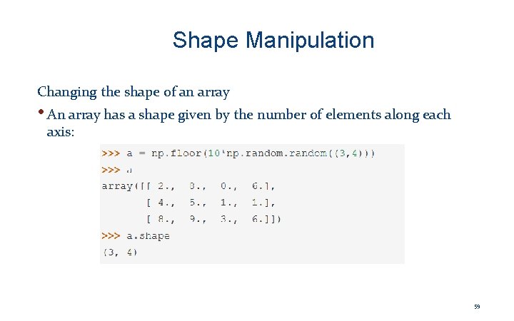
Shape Manipulation Changing the shape of an array • An array has a shape given by the number of elements along each axis: 59

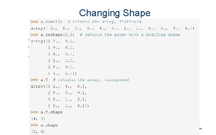
Changing Shape The shape of an array can be changed with various commands. The following commands return a modified array, but do not change the original array: 60

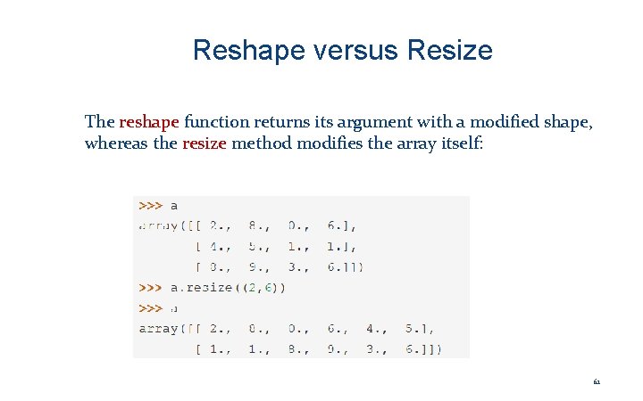
Reshape versus Resize The reshape function returns its argument with a modified shape, whereas the resize method modifies the array itself: 61

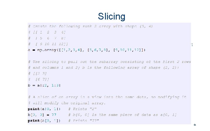
Slicing Similar to Python lists, numpy arrays can be sliced. Since arrays may be multidimensional, you must specify a slice for each dimension of the array: 62

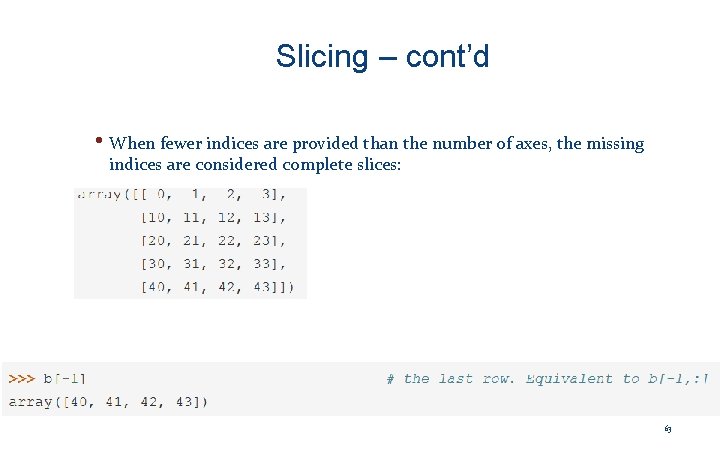
Slicing – cont’d • When fewer indices are provided than the number of axes, the missing indices are considered complete slices: 63

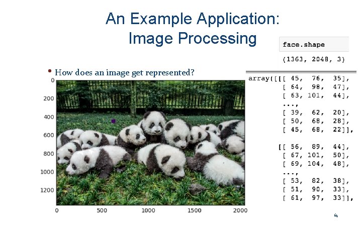
An Example Application: Image Processing • How does an image get represented? 64

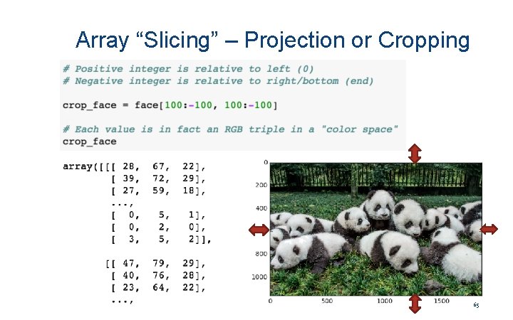
Array “Slicing” – Projection or Cropping 65

Beware: Numpy Slices Are NOT Copies • By default, a “slice” points to the data in the original array! • More efficient, but it means you need to be careful about changing the slice • i. e. , if I change values in crop_face, I also change face • If you’re going to modify the values, call array. copy() 66

Selecting Parts of an Array in Numpy 67

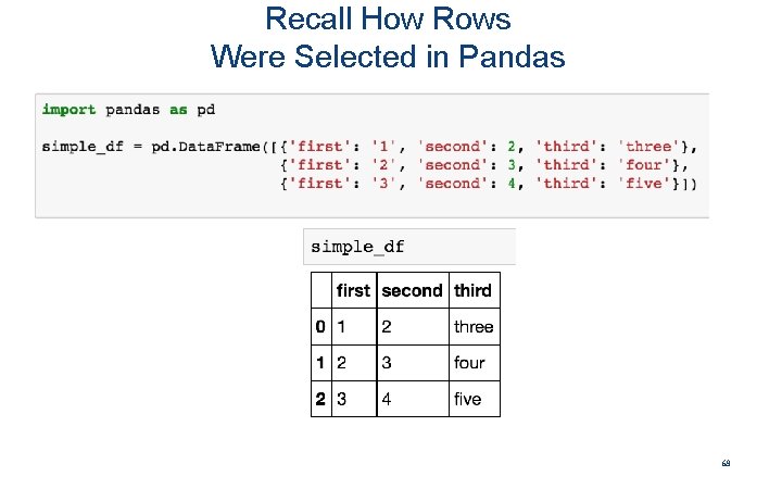
Recall How Rows Were Selected in Pandas 68

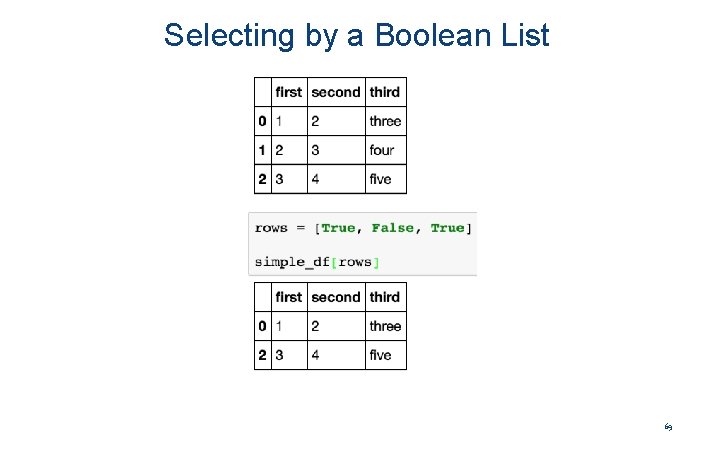
Selecting by a Boolean List 69

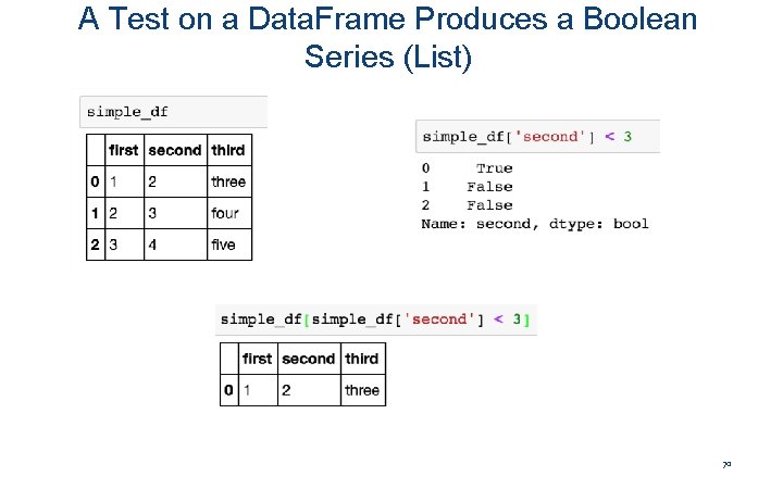
A Test on a Data. Frame Produces a Boolean Series (List) 70

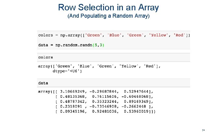
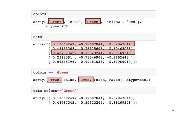
Row Selection in an Array (And Populating a Random Array) 71

72

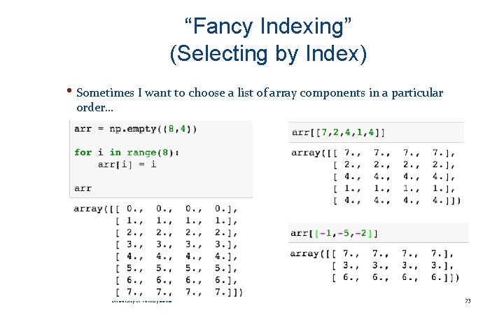
“Fancy Indexing” (Selecting by Index) • Sometimes I want to choose a list of array components in a particular order… University of Pennsylvania 73

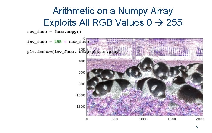
Arithmetic on a Numpy Array Exploits All RGB Values 0 255 74

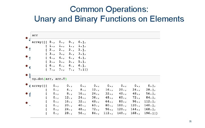
Common Operations: Unary and Binary Functions on Elements • abs • sqrt • square • exp • log • ceil • floor • … • add • subtract • multiply • power • mod • greater • dot 75

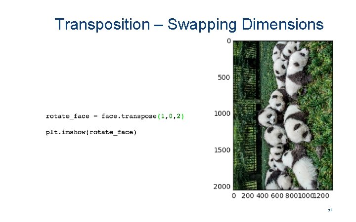
Transposition – Swapping Dimensions 76

Putting It Together 77

Randomly populating values • Create array with random values from distributions: • np. random. randn() – normal distribution with mean 0, stdev 1 • binomial • normal / Gaussian • beta • chisquare • gamma 78

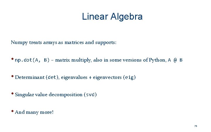
Linear Algebra Numpy treats arrays as matrices and supports: • np. dot(A, B) – matrix multiply, also in some versions of Python, A @ B • Determinant (det), eigenvalues + eigenvectors (eig) • Singular value decomposition (svd) • And many more! 79

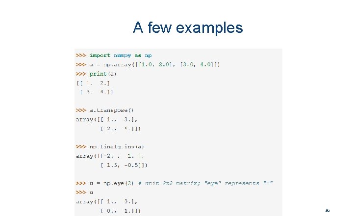
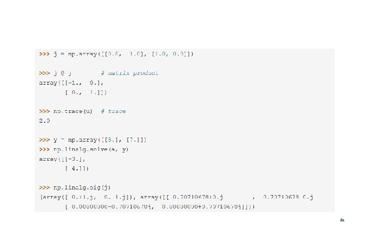
A few examples 80

81

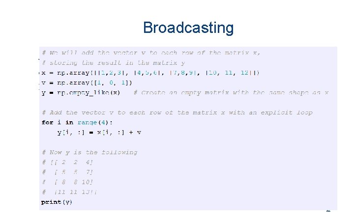
Broadcasting Work with arrays of different shapes when performing arithmetic operations Example: add a constant vector to each row of a matrix 82

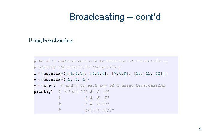
Broadcasting – cont’d Using broadcasting 83

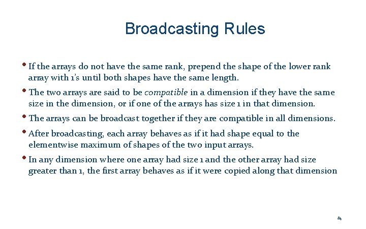
Broadcasting Rules • If the arrays do not have the same rank, prepend the shape of the lower rank array with 1’s until both shapes have the same length. • The two arrays are said to be compatible in a dimension if they have the same size in the dimension, or if one of the arrays has size 1 in that dimension. • The arrays can be broadcast together if they are compatible in all dimensions. • After broadcasting, each array behaves as if it had shape equal to the elementwise maximum of shapes of the two input arrays. • In any dimension where one array had size 1 and the other array had size greater than 1, the first array behaves as if it were copied along that dimension 84

Recap and Take-aways • Num. Py (and Sci. Py) provide powerful support for arrays and matrices • Bulk operators across the various elements, different kinds of iteration, … • For some kinds of array computations, there is a natural mapping to Spark -style distributed computation • . . . but for others we don’t get much speedup • Thus, we can do general-purpose matrix computation on a single machine, and specialized matrix computation in Spark • Sometimes it makes as much sense to encode the matrix data as a Data. Frame as a Spark matrix. . . 85