Data Intensive and Cloud Computing Graphs and Networks

Data Intensive and Cloud Computing Graphs and Networks Lecture 8 Slides based on Zack Ives / Clayton Greenberg at University of Pennsylvania

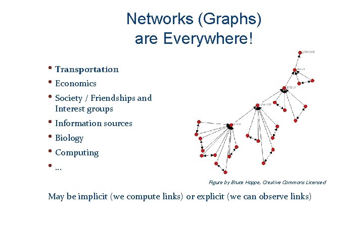
Networks (Graphs) are Everywhere! • Transportation • Economics • Society / Friendships and Interest groups • Information sources • Biology • Computing • . . . Figure by Bruce Hoppe, Creative Commons Licensed May be implicit (we compute links) or explicit (we can observe links)

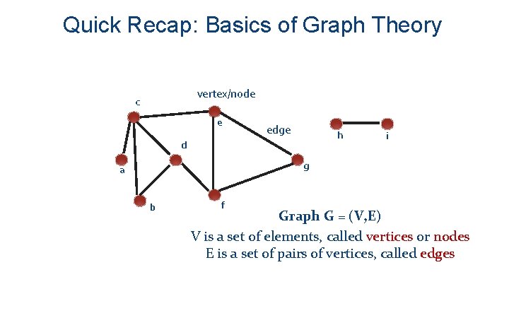
Quick Recap: Basics of Graph Theory vertex/node c e edge h d i g a b f Graph G = (V, E) V is a set of elements, called vertices or nodes E is a set of pairs of vertices, called edges

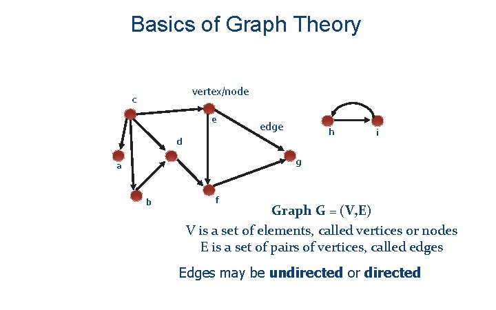
Basics of Graph Theory vertex/node c e edge h d i g a b f Graph G = (V, E) V is a set of elements, called vertices or nodes E is a set of pairs of vertices, called edges Edges may be undirected or directed

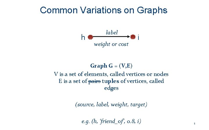
Common Variations on Graphs h label weight or cost i Graph G = (V, E) V is a set of elements, called vertices or nodes E is a set of pairs tuples of vertices, called edges (source, label, weight, target) e. g. (h, ‘friend_of’, 0. 8, i) 5

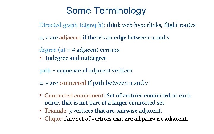
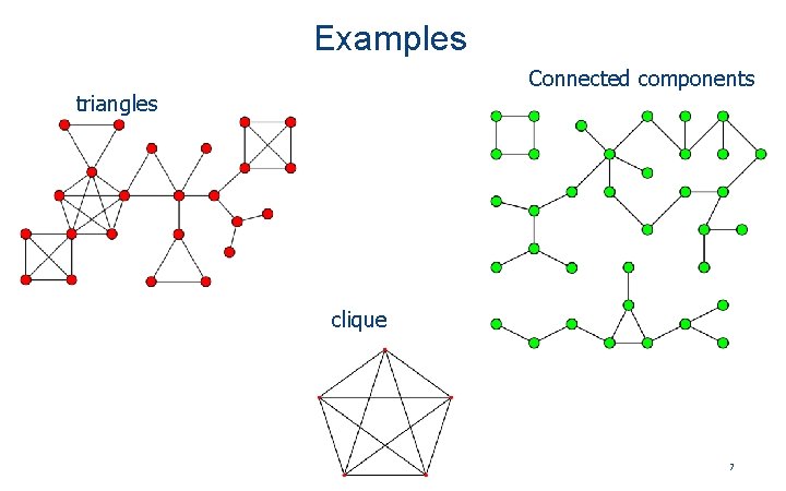
Some Terminology Directed graph (digraph): think web hyperlinks, flight routes u, v are adjacent if there’s an edge between u and v degree (u) = # adjacent vertices • indegree and outdegree path = sequence of adjacent vertices u, v are connected if path between u and v • Connected component: Set of vertices connected to each other, that is not part of a larger connected set. • Triangle: 3 vertices that are pairwise adjacent. • Clique: Any set of vertices that are all pairwise adjacent.

Examples Connected components triangles clique 7

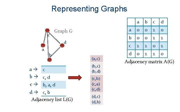
Representing Graphs c Graph G d a b a c b c, d c b, a, d d c, b Adjacency list L(G) (a, c) (b, d) (c, b) (c, a) (c, d) (d, c) (d, b) a b c d a 0 0 1 0 b 0 0 1 1 c 1 1 0 1 d 0 1 1 0 Adjacency matrix A(G)

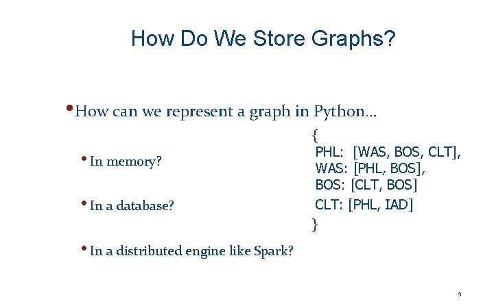
How Do We Store Graphs? • How can we represent a graph in Python… • In memory? • In a database? { PHL: [WAS, BOS, CLT], WAS: [PHL, BOS], BOS: [CLT, BOS] CLT: [PHL, IAD] } • In a distributed engine like Spark? 9

Graph Algorithms 10

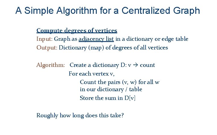
A Simple Algorithm for a Centralized Graph Compute degrees of vertices Input: Graph as adjacency list in a dictionary or edge table Output: Dictionary (map) of degrees of all vertices Algorithm: Create a dictionary D: v count For each vertex v, Count the pairs (v, w) for all w in our dictionary / table Store the sum in D[v] Roughly how long does this take?

Our Flights Example { PHL: [WAS, BOS, CLT], WAS: [PHL, BOS], BOS: [CLT, BOS] CLT: [PHL, IAD] } Create a dictionary D: v count For each vertex v, Count the pairs (v, w) for all w in our dictionary Store the sum in D[v] 12

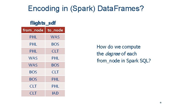
Encoding in (Spark) Data. Frames? flights_sdf from_node to_node PHL WAS PHL BOS PHL CLT WAS PHL WAS BOS CLT BOS PHL CLT IAD How do we compute the degree of each from_node in Spark SQL? 13

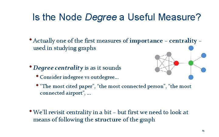
Is the Node Degree a Useful Measure? • Actually one of the first measures of importance – centrality – used in studying graphs • Degree centrality is as it sounds • Consider indegree vs outdegree… • “The most cited paper”, “the most connected person”, “the most connected airport”, … • We’ll revisit centrality in a bit – but first we need to look at means of following the structure of the graph 14

Graph Traversal 15

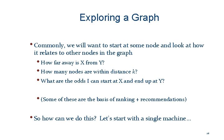
Exploring a Graph • Commonly, we will want to start at some node and look at how it relates to other nodes in the graph • How far away is X from Y? • How many nodes are within distance k? • What are the odds I can start at X and end up at Y? • (Some of these are the basis of ranking + recommendations) • So how can we do this? Let’s start with a single machine… 16

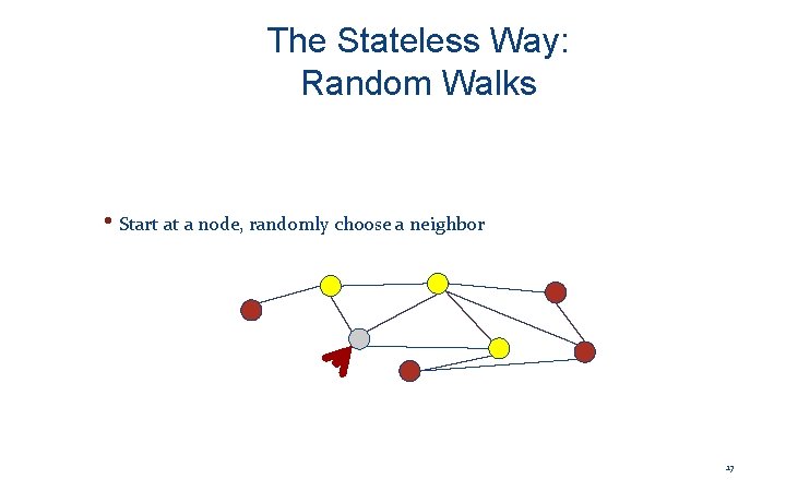
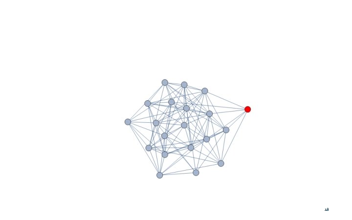
The Stateless Way: Random Walks • Start at a node, randomly choose a neighbor 17

18

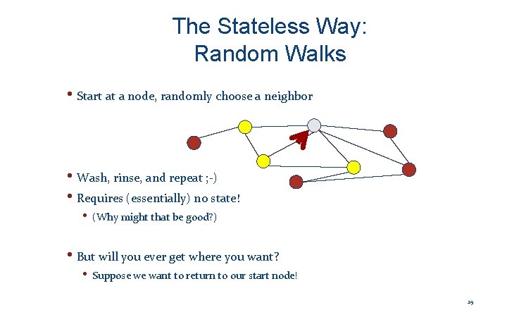
The Stateless Way: Random Walks • Start at a node, randomly choose a neighbor • Wash, rinse, and repeat ; -) • Requires (essentially) no state! • (Why might that be good? ) • But will you ever get where you want? • Suppose we want to return to our start node! 19

How Long Should We Expect It to Take to Traverse the Graph? • Given n nodes, m edges: • In expectation, we can start at node u, and visit and return from neighboring node v within 2 m steps (we won’t prove this here!) Revisit Markov Chains… • Thus we can estimate the time to visit all nodes: • E[Time to visit all nodes] <= 2 m (n-1) • Not surprisingly, that’s not great… Other ways? 20

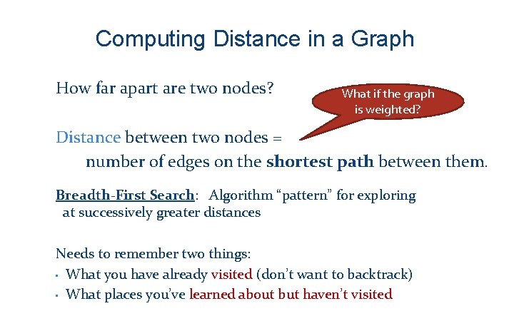
Computing Distance in a Graph How far apart are two nodes? What if the graph is weighted? Distance between two nodes = number of edges on the shortest path between them. Breadth-First Search: Algorithm “pattern” for exploring at successively greater distances Needs to remember two things: • What you have already visited (don’t want to backtrack) • What places you’ve learned about but haven’t visited

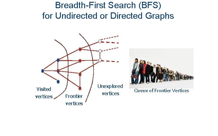
Breadth-First Search (BFS) for Undirected or Directed Graphs Visited vertices Frontier vertices Unexplored vertices Queue of Frontier Vertices

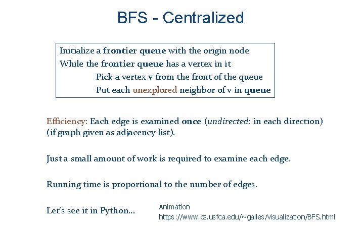
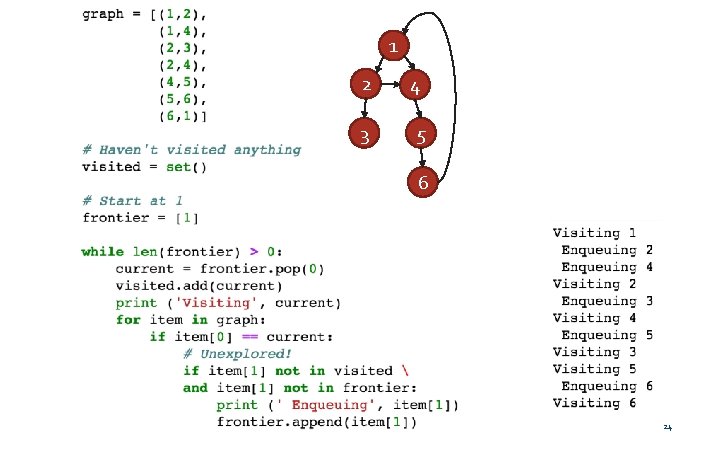
BFS - Centralized Initialize a frontier queue with the origin node While the frontier queue has a vertex in it Pick a vertex v from the front of the queue Put each unexplored neighbor of v in queue Efficiency: Each edge is examined once (undirected: in each direction) (if graph given as adjacency list). Just a small amount of work is required to examine each edge. Running time is proportional to the number of edges. Let’s see it in Python… Animation https: //www. cs. usfca. edu/~galles/visualization/BFS. html

1 2 4 3 5 6 24

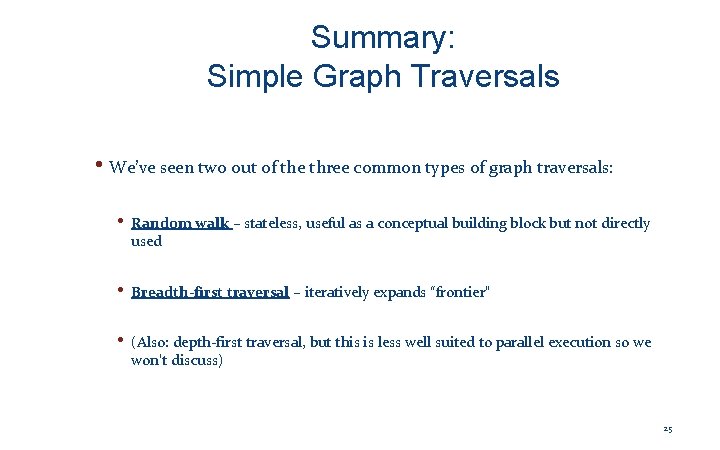
Summary: Simple Graph Traversals • We’ve seen two out of the three common types of graph traversals: • Random walk – stateless, useful as a conceptual building block but not directly used • Breadth-first traversal – iteratively expands “frontier” • (Also: depth-first traversal, but this is less well suited to parallel execution so we won’t discuss) 25

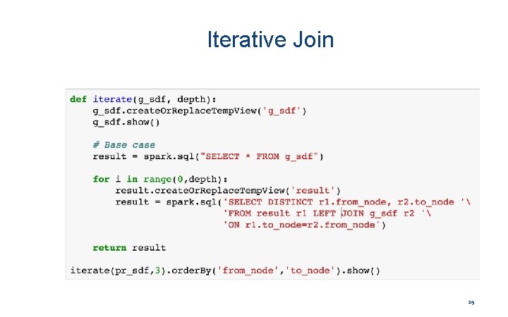
Graph Traversals in Spark: Iterative Joins! 26

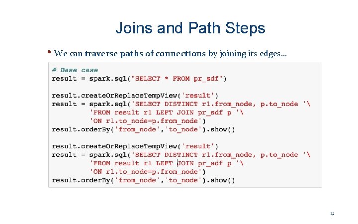
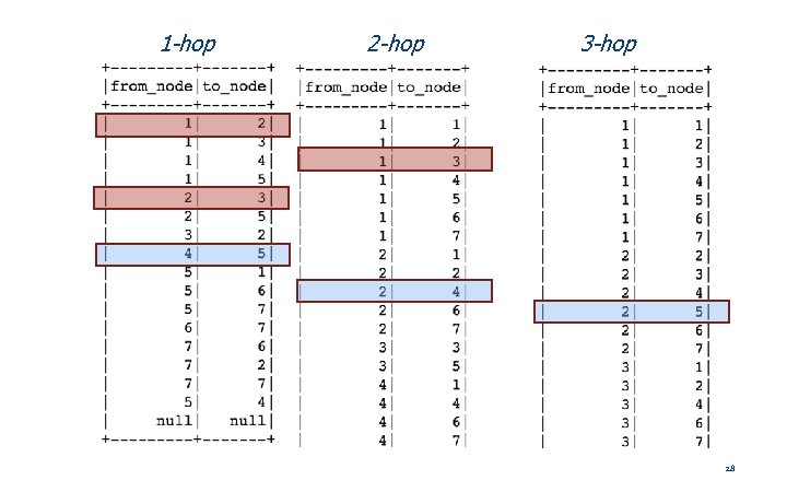
Joins and Path Steps • We can traverse paths of connections by joining its edges… 27

1 -hop 2 -hop 3 -hop 28

Iterative Join 29

From Here… • You have the building blocks to do quite rich algorithms! • We’ll start to look now at particular kinds of data beyond “mere” tables… • Starting with graphs (a generalization of the flight routes), then matrices. . . 30

A Few Applications of BFS 31

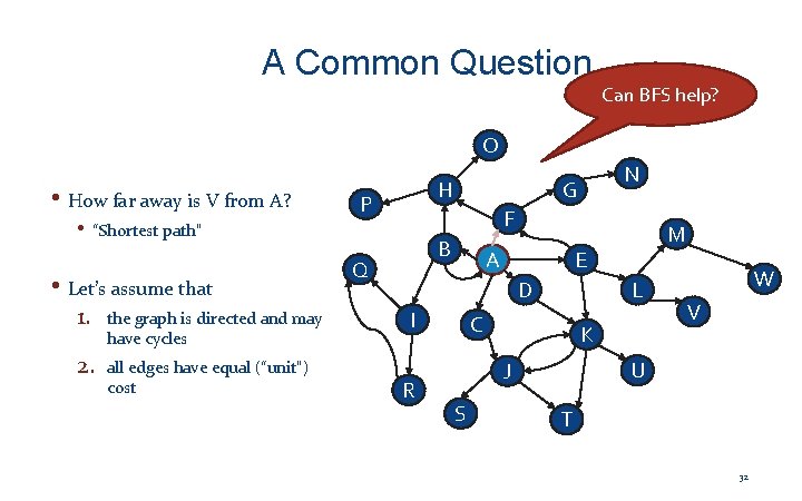
A Common Question Can BFS help? O • How far away is V from A? • “Shortest path” • Let’s assume that 1. the graph is directed and may have cycles 2. all edges have equal (“unit”) cost H P N G F B Q A E D I R L C K W V U J S M T 32

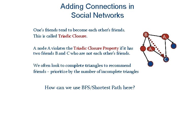
Adding Connections in Social Networks One’s friends tend to become each other’s friends. This is called Triadic Closure. A node A violates the Triadic Closure Property if it has two friends B and C who are not each other’s friends. B A 2 A 1 C We often look to complete triangles to recommend friends – prioritize by the number of incomplete triangles How can we use BFS/Shortest Path here?

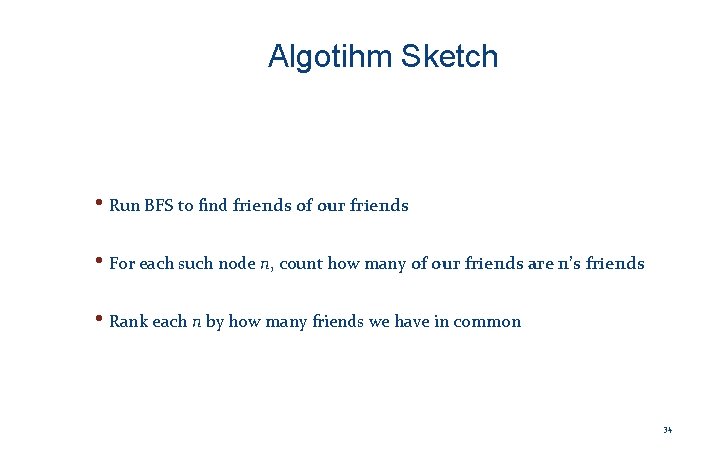
Algotihm Sketch • Run BFS to find friends of our friends • For each such node n, count how many of our friends are n’s friends • Rank each n by how many friends we have in common 34

Other Common Path-based algorithms • Sometimes our goal is to compute information about the paths (sets of paths) between nodes • Edges may be annotated with cost, distance, or similarity • Examples of such problems (see algorithms courses): • Shortest path from one node to another (we saw) • Minimum spanning tree (minimal-cost tree connecting all vertices in a graph) • Steiner tree (minimal-cost tree connecting certain nodes) • Topological sort (node in a graph without cycles comes before all nodes it points to) • Other times we want to visit all nodes, all edges, … 35

Summary – Breadth-First Search: A Useful Building Block • We’ve seen BFS in a single-computer world • And we’ve seen that it’s useful for computing shortest paths and for recommending friends • It’s also parallelizable on Spark / Map. Reduce etc. 36

Centrality and Page Rank 37

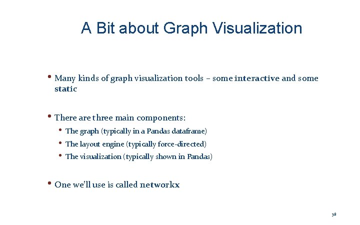
A Bit about Graph Visualization • Many kinds of graph visualization tools – some interactive and some static • There are three main components: • The graph (typically in a Pandas dataframe) • The layout engine (typically force-directed) • The visualization (typically shown in Pandas) • One we’ll use is called networkx 38

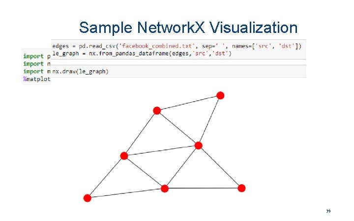
Sample Network. X Visualization 39

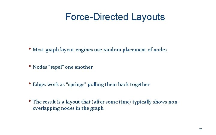
Force-Directed Layouts • Most graph layout engines use random placement of nodes • Nodes “repel” one another • Edges work as “springs” pulling them back together • The result is a layout that (after some time) typically shows nonoverlapping nodes in the graph 40

Importance 41

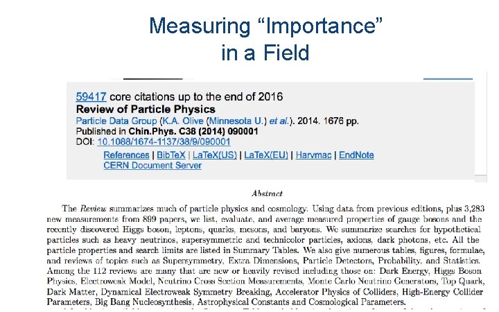
Measuring “Importance” in a Field • We saw that degree of a node tells how well connected it is – directly • But what about indirectly? • e. g. , how do we know Einstein was an influential physicist? University of Pennsylvania 42

Measuring “Importance” in a Graph • Different notions of centrality have been defined based on connectivity – • “betweenness centrality” measures how important a node is in bridging communities • eigenvector centrality gives us a recursive measure of importance, i. e. , do I connect to important nodes, do they connect to important nodes, etc. • In the Web graph, this is called link analysis 43

Link Analysis for the Web • Suppose a search engine processes a query for “physics" • Problem: Millions of pages contain these words! • Which ones should we return first? • Idea: Hyperlinks encode a considerable amount of human judgment, much as citations do • What does it mean when a web page links another page? • Intra-domain links: Often created primarily for navigation • Inter-domain links: Confer some measure of authority • It’s more than looking at the count of the links! 44

Other Applications of the Same Idea • This question occurs in several other areas: • How do we measure the "impact" of a researcher? (#papers? #citations? ) • What are the most useful datasets? (# downloads? ) • Who are the most "influential" individuals in a social network? (#friends? ) • Which programmers are writing the "best" code? (#uses? ) • . . . 45

Inventors Page rank 46

Intuition – (1) • Web pages are important if people visit them a lot. • But, can we watch everybody using the Web? • A good surrogate for visiting pages is to assume people follow links randomly. • Leads to random surfer model: • Start at a random page and follow random out-links repeatedly, from whatever page you are at. • Page. Rank = limiting probability of being at a page. 47

Intuition – (2) • Solve the recursive equation: a page is important to the extent that important pages link to it • Equivalent to the random-surfer definition of Page. Rank. • Technically, importance = the principal eigenvector of the transition matrix of the Web. • A few fixups needed. 48

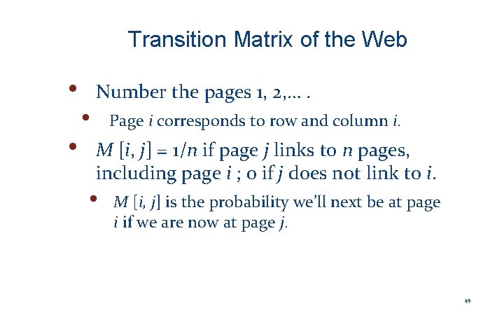
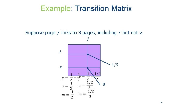
Transition Matrix of the Web • • • Number the pages 1, 2, …. Page i corresponds to row and column i. M [i, j] = 1/n if page j links to n pages, including page i ; 0 if j does not link to i. • M [i, j] is the probability we’ll next be at page i if we are now at page j. 49

Example: Transition Matrix Suppose page j links to 3 pages, including i but not x. j i 1/3 x 0 50

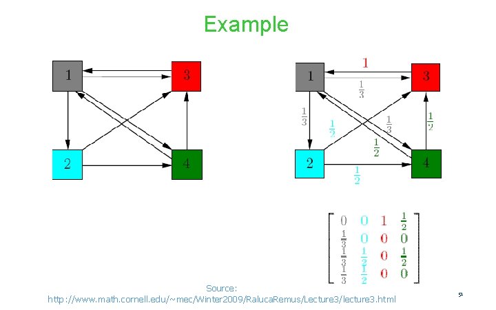
Example Source: http: //www. math. cornell. edu/~mec/Winter 2009/Raluca. Remus/Lecture 3/lecture 3. html 51

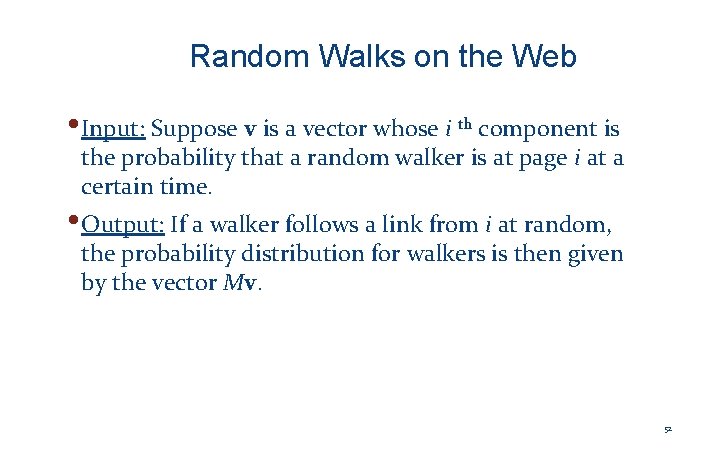
Random Walks on the Web • Input: Suppose v is a vector whose i th component is the probability that a random walker is at page i at a certain time. • Output: If a walker follows a link from i at random, the probability distribution for walkers is then given by the vector Mv. 52

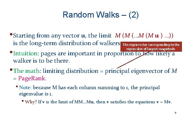
Random Walks – (2) • Starting from any vector u, the limit M (M (…M (M u ) …)) is the long-term distribution of walkers. The eigenvector corresponding to the eigenvalue of largest magnitude. • Intuition: pages are important in proportion to how likely a walker is to be there. • The math: limiting distribution = principal eigenvector of M = Page. Rank. • Note: because M has each column summing to 1, the principal eigenvalue is 1. • Why? If v is the limit of MM…Mu, then v satisfies the equations v = Mv. 53

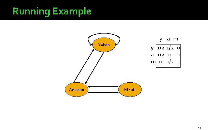
Running Example y a m Yahoo Amazon y 1/2 0 a 1/2 0 1 m 0 1/2 0 M’soft 54

Solving The Equations • Because there are no constant terms, the equations v = Mv do not have a unique solution. • In Web-sized examples, we cannot solve by Gaussian elimination anyway; we need to use relaxation (= iterative solution). • Works if you start with any nonzero u. 55

Simulating a Random Walk • Start with the vector u = [1, 1, …, 1] representing the idea that each Web page is given one unit of importance. • Note: it is more common to start with each vector element = 1/n, where n is the number of Web pages. • Repeatedly apply the matrix M to u, allowing the importance to flow like a random walk. • About 50 iterations is sufficient to estimate the limiting solution. 56

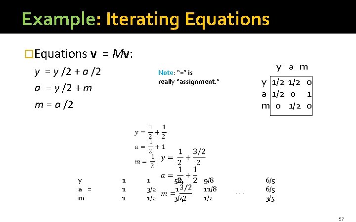
Example: Iterating Equations �Equations v = Mv: y = y /2 + a /2 a = y /2 + m m = a /2 y a = m y a m Note: “=” is really “assignment. ” 1 1 3/2 1/2 5/4 1 3/4 9/8 11/8 1/2 y 1/2 0 a 1/2 0 1 m 0 1/2 0 . . . 6/5 3/5 57

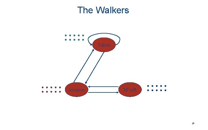
The Walkers Yahoo Amazon M’soft 58

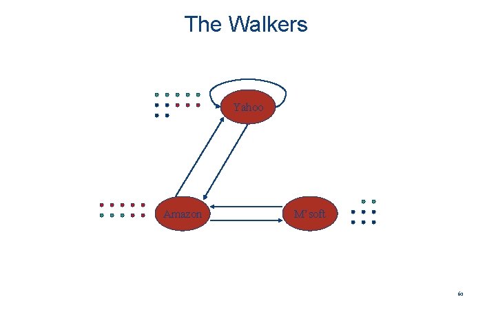
The Walkers Yahoo Amazon M’soft 59

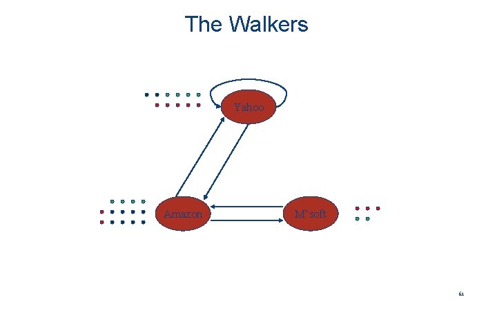
The Walkers Yahoo Amazon M’soft 60

The Walkers Yahoo Amazon M’soft 61

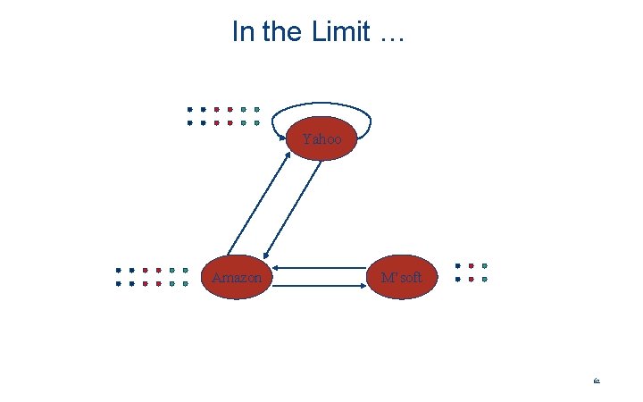
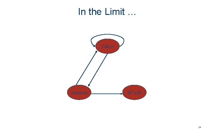
In the Limit … Yahoo Amazon M’soft 62

The Web Is More Complex Than That Dead Ends Spider Traps Taxation Policies

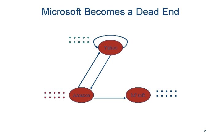
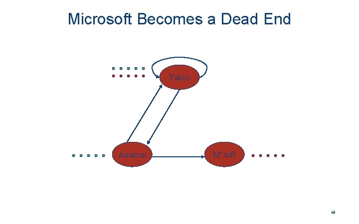
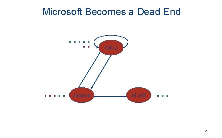
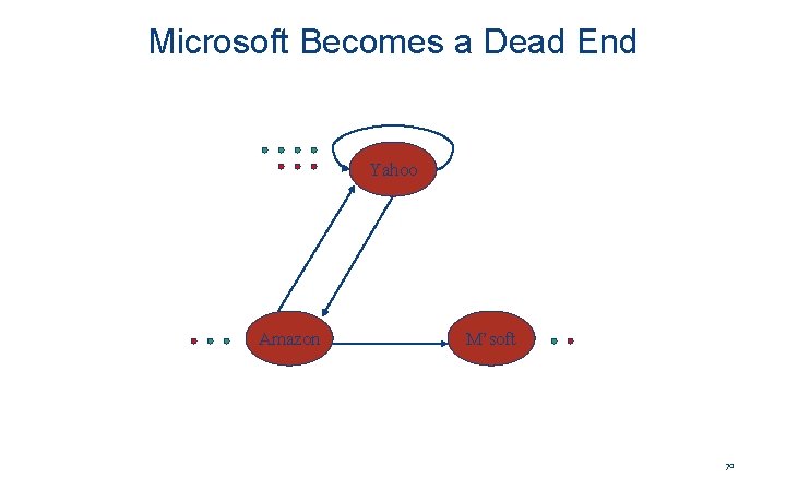
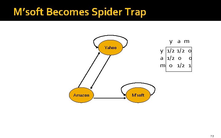
Real-World Problems • Some pages are dead ends (have no links out). • Such a page causes importance to leak out. • Other groups of pages are spider traps (all outlinks are within the group). • Eventually spider traps absorb all importance. 64

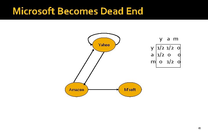
Microsoft Becomes Dead End y a m Yahoo Amazon y 1/2 0 a 1/2 0 0 m 0 1/2 0 M’soft 65

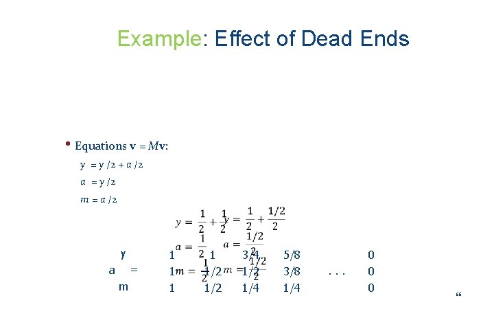
Example: Effect of Dead Ends • Equations v = Mv: y = y /2 + a /2 a = y /2 m = a /2 y a = m 1 1 1/2 3/4 1/2 1/4 5/8 3/8 1/4 . . . 0 0 0 66

Microsoft Becomes a Dead End Yahoo Amazon M’soft 67

Microsoft Becomes a Dead End Yahoo Amazon M’soft 68

Microsoft Becomes a Dead End Yahoo Amazon M’soft 69

Microsoft Becomes a Dead End Yahoo Amazon M’soft 70

In the Limit … Yahoo Amazon M’soft 71

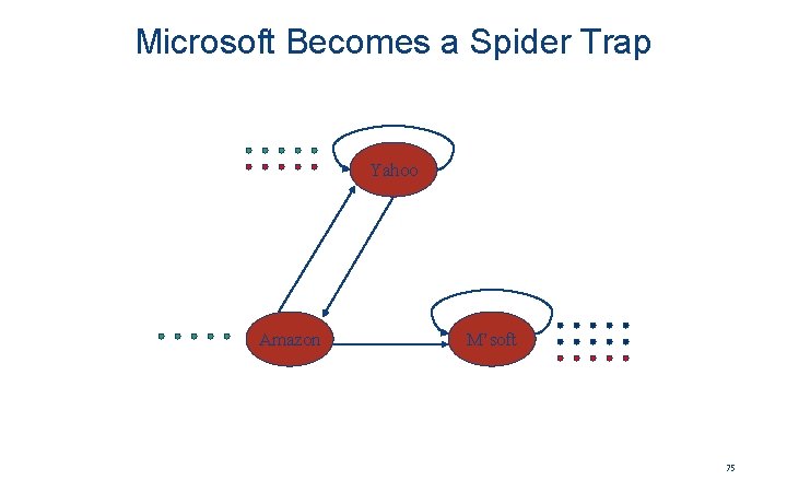
M’soft Becomes Spider Trap y a m Yahoo Amazon y 1/2 0 a 1/2 0 0 m 0 1/2 1 M’soft 72

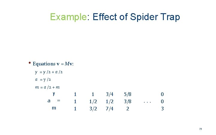
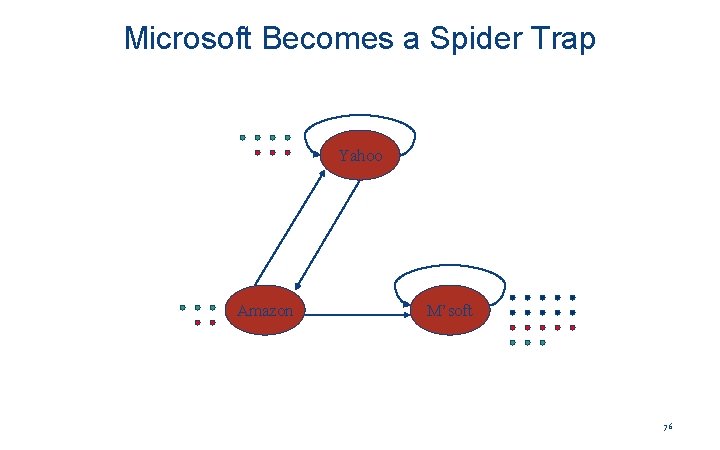
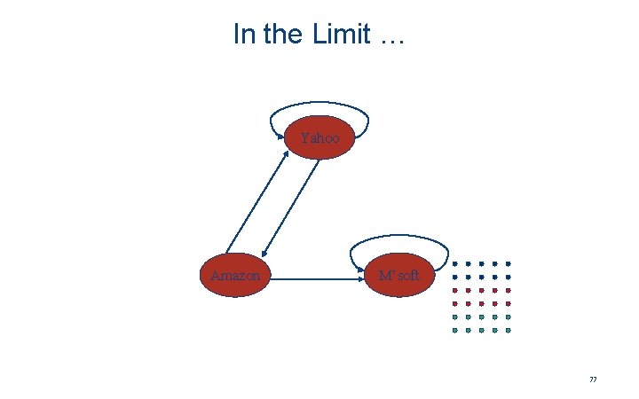
Example: Effect of Spider Trap • Equations v = Mv: y = y /2 + a /2 a = y /2 m = a /2 + m y a = m 1 1 1/2 3/4 1/2 7/4 5/8 3/8 2 . . . 0 0 3 73

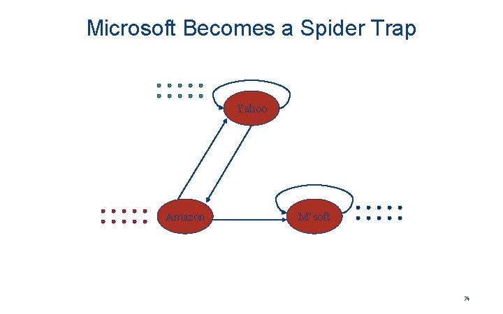
Microsoft Becomes a Spider Trap Yahoo Amazon M’soft 74

Microsoft Becomes a Spider Trap Yahoo Amazon M’soft 75

Microsoft Becomes a Spider Trap Yahoo Amazon M’soft 76

In the Limit … Yahoo Amazon M’soft 77

Page. Rank Solution to Traps, Etc. • “Tax” each page a fixed percentage at each iteration. • Add a fixed constant to all pages. • Optional but useful: add exactly enough to balance the loss (tax + Page. Rank of dead ends). • Models a random walk with a fixed probability of leaving the system, and a fixed number of new walkers injected into the system at each step. • Divided equally among all pages. 78

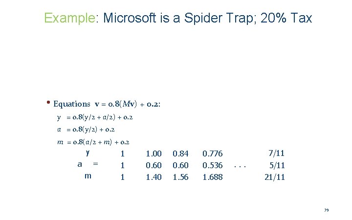
Example: Microsoft is a Spider Trap; 20% Tax • Equations v = 0. 8(Mv) + 0. 2: y = 0. 8(y/2 + a/2) + 0. 2 a = 0. 8(y/2) + 0. 2 m = 0. 8(a/2 + m) + 0. 2 y a = m 1 1. 00 0. 60 1. 40 0. 84 0. 60 1. 56 0. 776 0. 536 1. 688 . . . 7/11 5/11 21/11 79

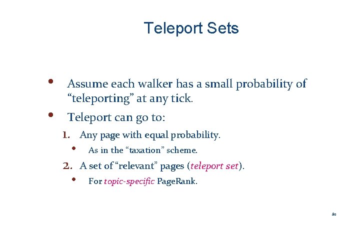
Teleport Sets • • Assume each walker has a small probability of “teleporting” at any tick. Teleport can go to: 1. Any page with equal probability. • 2. • As in the “taxation” scheme. A set of “relevant” pages (teleport set). For topic-specific Page. Rank. 80

Application: Link Spam • Spam farmers create networks of millions of pages designed to focus Page. Rank on a few undeserving pages. • To minimize their influence, use a teleport set consisting of trusted pages only. • Example: home pages of universities. 81

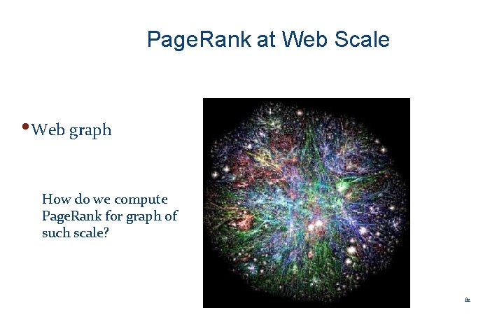
Page. Rank at Web Scale • Web graph How do we compute Page. Rank for graph of such scale? 82

Implementing Naïve Page. Rank 83

Great! We Can Compute Page. Rank Iteratively • e. g. , using the recursive join computations we saw for Spark • But some pieces of this can be thought of in a more general way 84

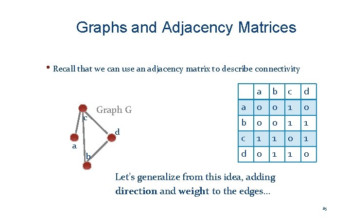
Graphs and Adjacency Matrices • Recall that we can use an adjacency matrix to describe connectivity c Graph G d a b c d a 0 0 1 0 b 0 0 1 1 c 1 1 0 1 d 0 1 1 0 Let’s generalize from this idea, adding direction and weight to the edges… 85

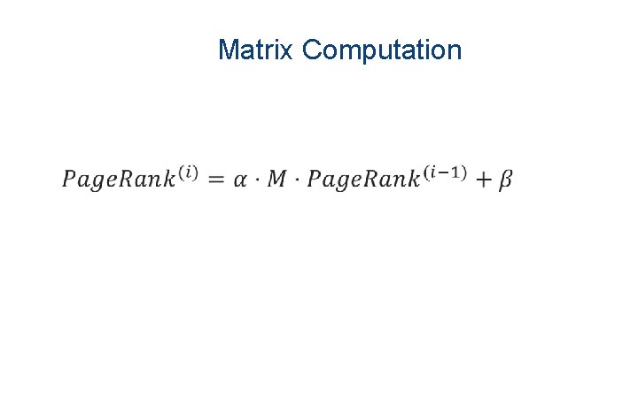
Matrix Computation

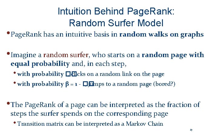
Intuition Behind Page. Rank: Random Surfer Model • Page. Rank has an intuitive basis in random walks on graphs • Imagine a random surfer, who starts on a random page with equal probability and, in each step, • with probability �� , clicks on a random link on the page • with probability β = 1 - �� , jumps to a random page (bored? ) • The Page. Rank of a page can be interpreted as the fraction of steps the surfer spends on the corresponding page • Transition matrix can be interpreted as a Markov Chain 87

Variations on Page. Rank • Many have been studied! • What if we don’t randomly jump with equal probability? • What if we want to “personalize” Page. Rank or measure it relative to certain start points? 88

Recap and Take-aways • We’ve seen some basic algorithms for graphs – which are incredibly common in representing real-world phenomena • Later we’ll see how we can build graphs representing similarities / overlap among data • Next let’s see how to use Python’s support for matrices to implement Page. Rank… and a few other things! 89