Data in MATLAB lesson 2 T Jehl Variables

Data in MATLAB lesson 2 T Jehl

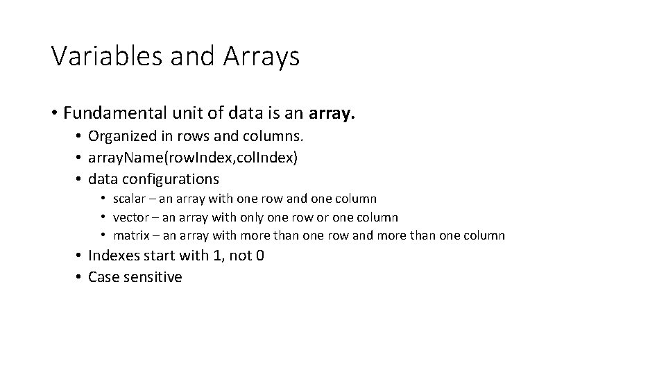
Variables and Arrays • Fundamental unit of data is an array. • Organized in rows and columns. • array. Name(row. Index, col. Index) • data configurations • scalar – an array with one row and one column • vector – an array with only one row or one column • matrix – an array with more than one row and more than one column • Indexes start with 1, not 0 • Case sensitive

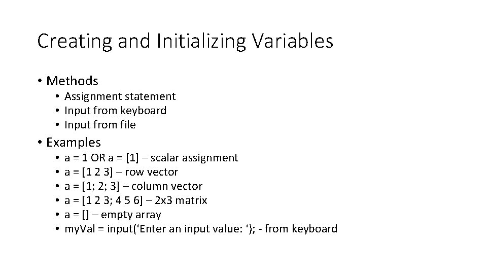
Creating and Initializing Variables • Methods • Assignment statement • Input from keyboard • Input from file • Examples • • • a = 1 OR a = [1] – scalar assignment a = [1 2 3] – row vector a = [1; 2; 3] – column vector a = [1 2 3; 4 5 6] – 2 x 3 matrix a = [] – empty array my. Val = input(‘Enter an input value: ‘); - from keyboard

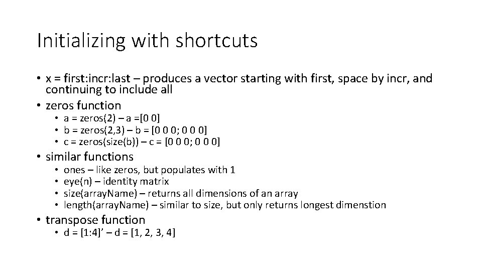
Initializing with shortcuts • x = first: incr: last – produces a vector starting with first, space by incr, and continuing to include all • zeros function • a = zeros(2) – a =[0 0] • b = zeros(2, 3) – b = [0 0 0; 0 0 0] • c = zeros(size(b)) – c = [0 0 0; 0 0 0] • similar functions • • ones – like zeros, but populates with 1 eye(n) – identity matrix size(array. Name) – returns all dimensions of an array length(array. Name) – similar to size, but only returns longest dimenstion • transpose function • d = [1: 4]’ – d = [1, 2, 3, 4]

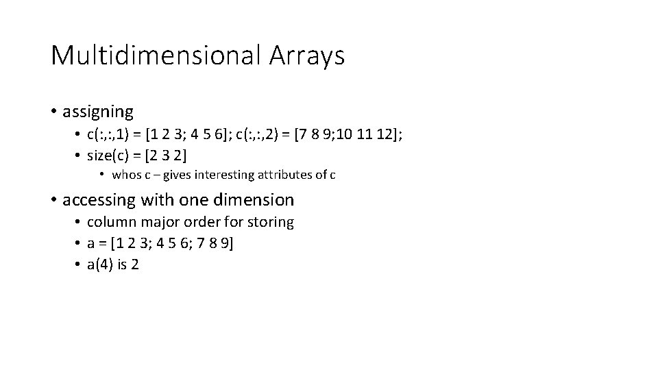
Multidimensional Arrays • assigning • c(: , 1) = [1 2 3; 4 5 6]; c(: , 2) = [7 8 9; 10 11 12]; • size(c) = [2 3 2] • whos c – gives interesting attributes of c • accessing with one dimension • column major order for storing • a = [1 2 3; 4 5 6; 7 8 9] • a(4) is 2

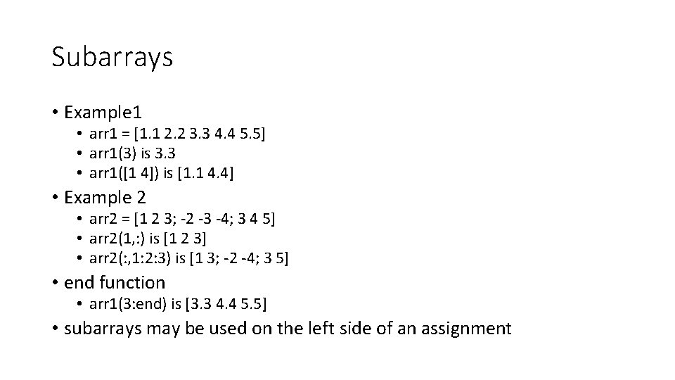
Subarrays • Example 1 • arr 1 = [1. 1 2. 2 3. 3 4. 4 5. 5] • arr 1(3) is 3. 3 • arr 1([1 4]) is [1. 1 4. 4] • Example 2 • arr 2 = [1 2 3; -2 -3 -4; 3 4 5] • arr 2(1, : ) is [1 2 3] • arr 2(: , 1: 2: 3) is [1 3; -2 -4; 3 5] • end function • arr 1(3: end) is [3. 3 4. 4 5. 5] • subarrays may be used on the left side of an assignment

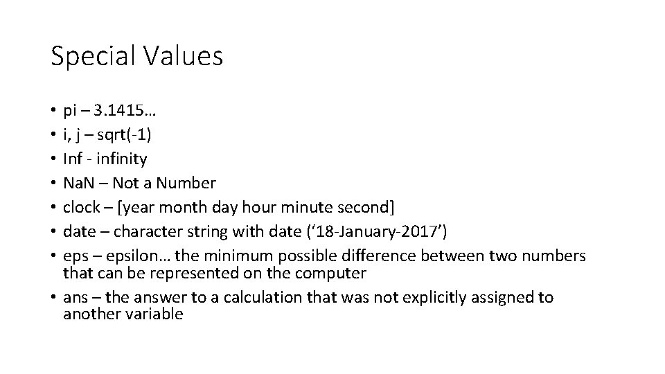
Special Values pi – 3. 1415… i, j – sqrt(-1) Inf - infinity Na. N – Not a Number clock – [year month day hour minute second] date – character string with date (‘ 18 -January-2017’) eps – epsilon… the minimum possible difference between two numbers that can be represented on the computer • ans – the answer to a calculation that was not explicitly assigned to another variable • •

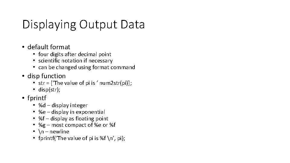
Displaying Output Data • default format • four digits after decimal point • scientific notation if necessary • can be changed using format command • disp function • str = [‘The value of pi is ‘ num 2 str(pi)]; • disp(str); • fprintf • • • %d – display integer %e – display in exponential %f – display as floating point %g – most compact of %e or %f n – newline fprintf(‘The value of pi is %f n’, pi);

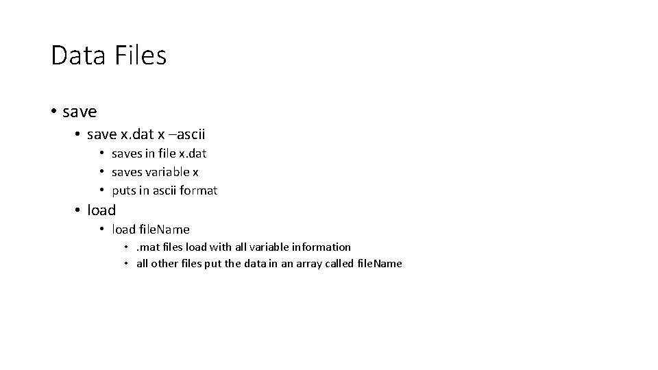
Data Files • save x. dat x –ascii • saves in file x. dat • saves variable x • puts in ascii format • load file. Name • . mat files load with all variable information • all other files put the data in an array called file. Name

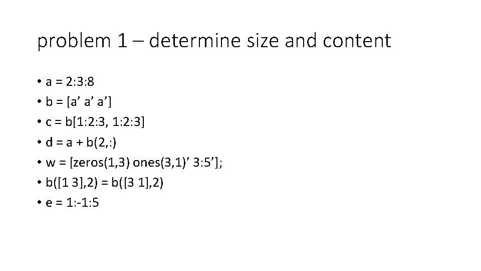
problem 1 – determine size and content • a = 2: 3: 8 • b = [a’ a’ a’] • c = b[1: 2: 3, 1: 2: 3] • d = a + b(2, : ) • w = [zeros(1, 3) ones(3, 1)’ 3: 5’]; • b([1 3], 2) = b([3 1], 2) • e = 1: -1: 5

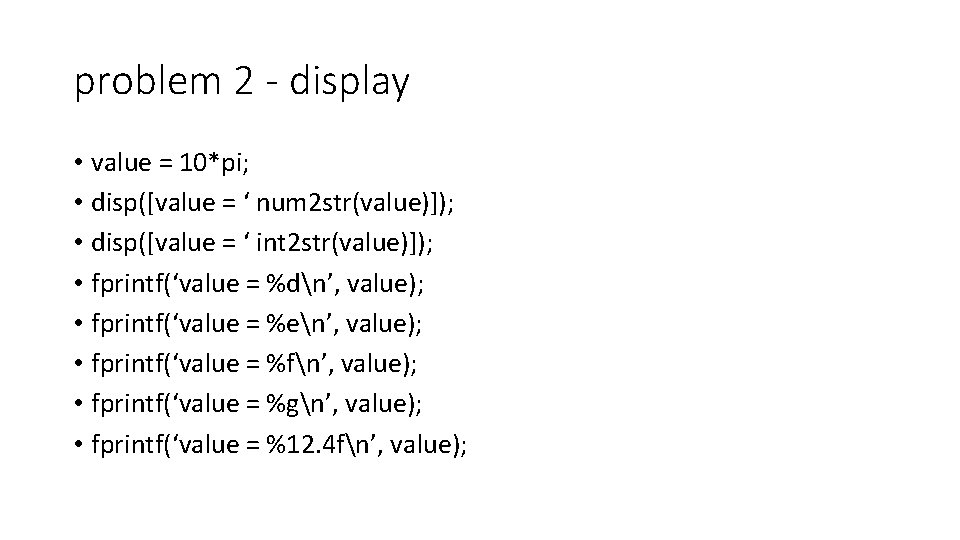
problem 2 - display • value = 10*pi; • disp([value = ‘ num 2 str(value)]); • disp([value = ‘ int 2 str(value)]); • fprintf(‘value = %dn’, value); • fprintf(‘value = %en’, value); • fprintf(‘value = %fn’, value); • fprintf(‘value = %gn’, value); • fprintf(‘value = %12. 4 fn’, value);