Data Assimilation Training Course Final Discussion and QA

Data Assimilation Training Course Final Discussion and Q&A 1

Data Assimilation has two main goals: – Optimally blend information from observations and model to produce an accurate and physically consistent estimate of the initial state of the atmosphere and of the other components of the Earth System – Quantify the uncertainty of our estimate of the initial state (this is necessary to be able to initialise an ensemble forecast!) 2

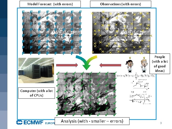
Model Forecast (with errors) Observations (with errors) People (with a lot of good ideas) Computer (with a lot of CPUs) Analysis (with - smaller – errors) 3

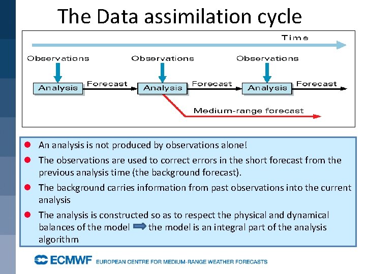
The Data assimilation cycle l An analysis is not produced by observations alone! l The observations are used to correct errors in the short forecast from the previous analysis time (the background forecast). l The background carries information from past observations into the current analysis l The analysis is constructed so as to respect the physical and dynamical balances of the model is an integral part of the analysis algorithm

The observations

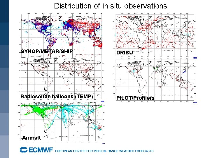
Distribution of in situ observations SYNOP/METAR/SHIP DRIBU Radiosonde balloons (TEMP) PILOT/Profilers Aircraft

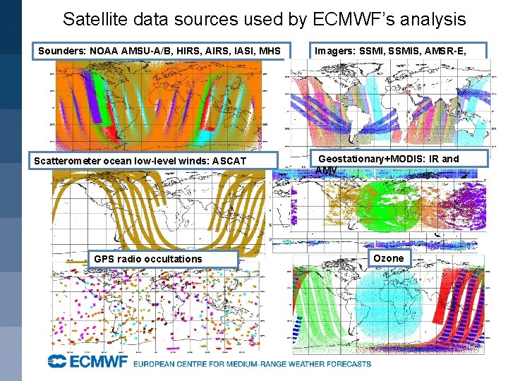
Satellite data sources used by ECMWF’s analysis Sounders: NOAA AMSU-A/B, HIRS, AIRS, IASI, MHS Scatterometer ocean low-level winds: ASCAT GPS radio occultations Imagers: SSMI, SSMIS, AMSR-E, TMI Geostationary+MODIS: IR and AMV Ozone

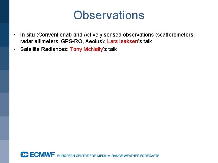
Observations • In situ (Conventional) and Actively sensed observations (scatterometers, radar altimeters, GPS-RO, Aeolus): Lars Isaksen’s talk • Satellite Radiances: Tony Mc. Nally’s talk

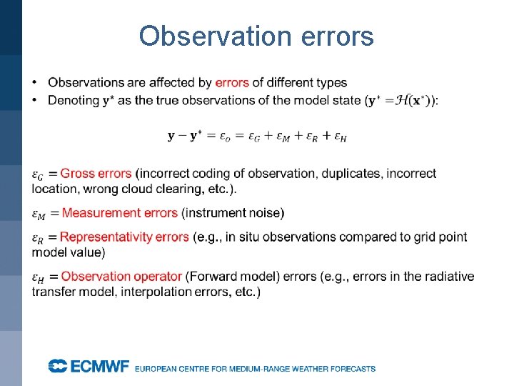
Observation errors

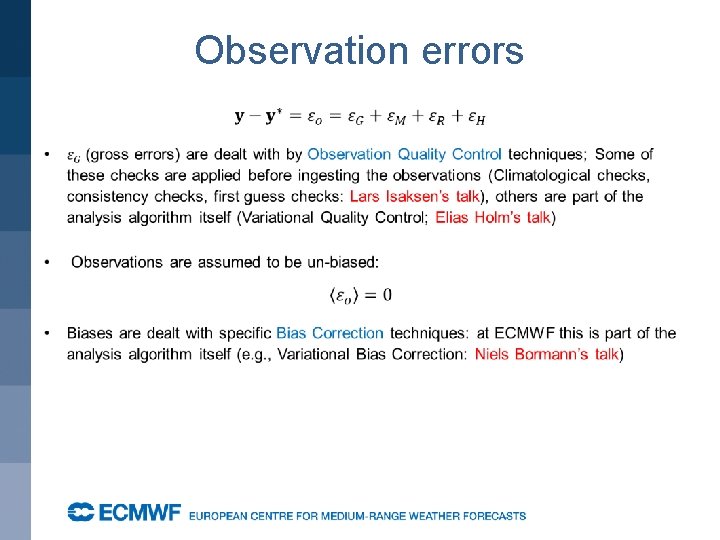
Observation errors

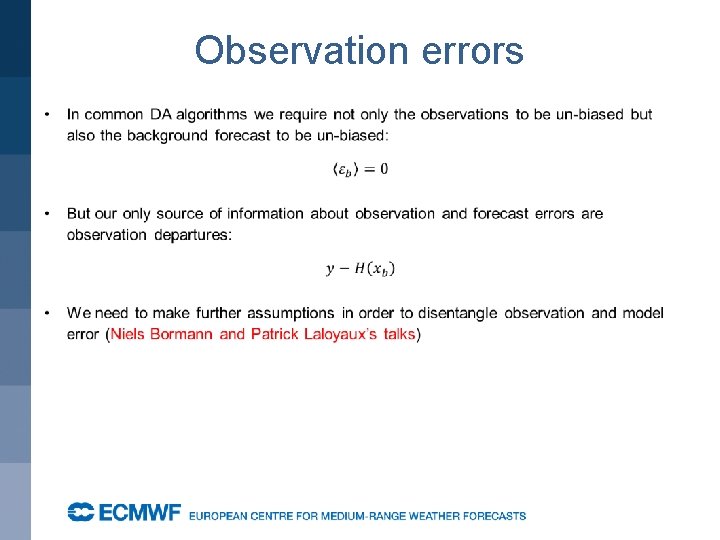
Observation errors

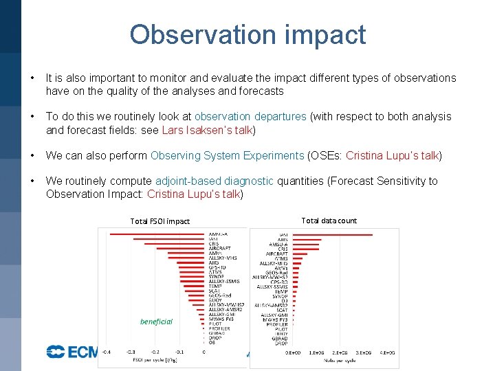
Observation impact • It is also important to monitor and evaluate the impact different types of observations have on the quality of the analyses and forecasts • To do this we routinely look at observation departures (with respect to both analysis and forecast fields: see Lars Isaksen’s talk) • We can also perform Observing System Experiments (OSEs: Cristina Lupu’s talk) • We routinely compute adjoint-based diagnostic quantities (Forecast Sensitivity to Observation Impact: Cristina Lupu’s talk) Total FSOI impact beneficial Total data count

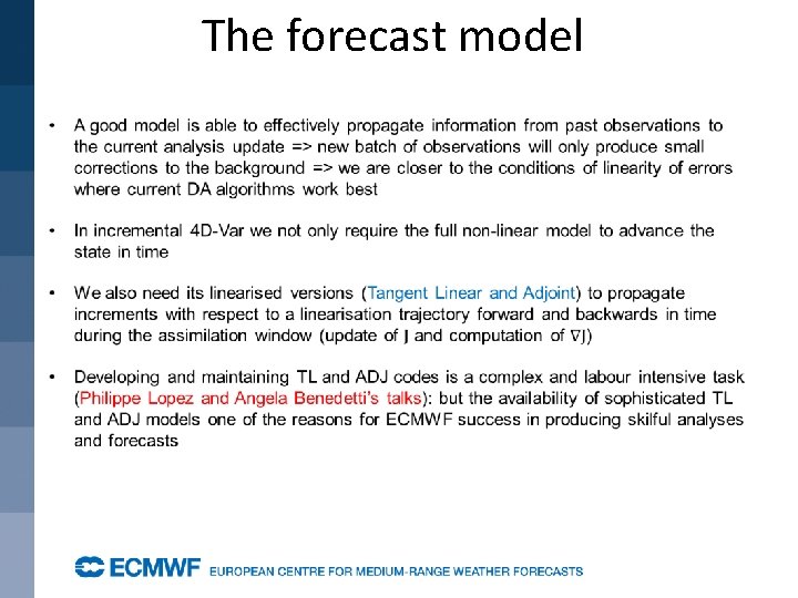
The forecast model

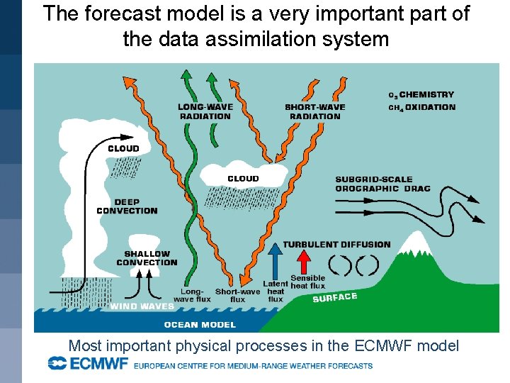
The forecast model is a very important part of the data assimilation system Most important physical processes in the ECMWF model

The forecast model

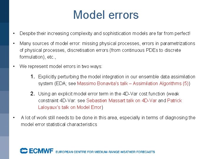
Model errors • Despite their increasing complexity and sophistication models are far from perfect! • Many sources of model error: missing physical processes, errors in parametrizations of physical processes, discretisation errors (from continuous PDEs to discrete formulation), etc. , • We represent model errors in two ways: 1. Explicitly perturbing the model integration in our ensemble data assimilation system (EDA; see Massimo Bonavita’s talk – Assimilation Algorithms (5)) 2. Using an explicit model error term in the 4 D-Var cost function (weak constraint 4 D-Var: see Sebastien Massart talk on 4 D-Var and Patrick Laloyaux’s talk on Model Error) • A lot of work still needs to be done in this area, especially in terms of diagnosing the model error statistical characteristics

Blending observations and model information: the Bayes perspective 17

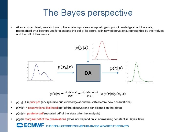
The Bayes perspective DA

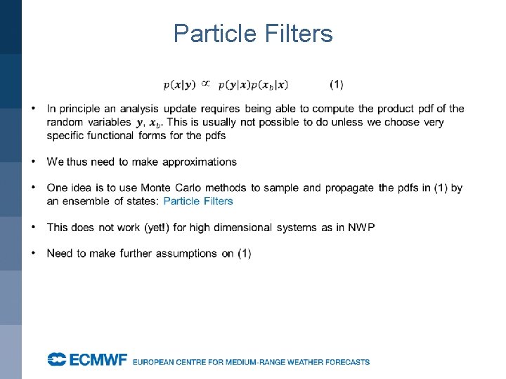
Particle Filters

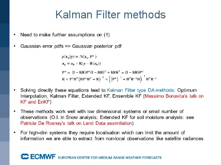
Kalman Filter methods

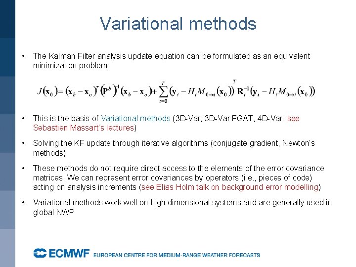
Variational methods • The Kalman Filter analysis update equation can be formulated as an equivalent minimization problem: • This is the basis of Variational methods (3 D-Var, 3 D-Var FGAT, 4 D-Var: see Sebastien Massart’s lectures) • Solving the KF update through iterative algorithms (conjugate gradient, Newton’s methods) • These methods do not require direct access to the elements of the error covariance matrices. We can represent error covariances by operators (i. e. , pieces of code) acting on analysis increments (see Elias Holm talk on background error modelling) • Variational methods work well on high dimensional systems and are generally used in global NWP

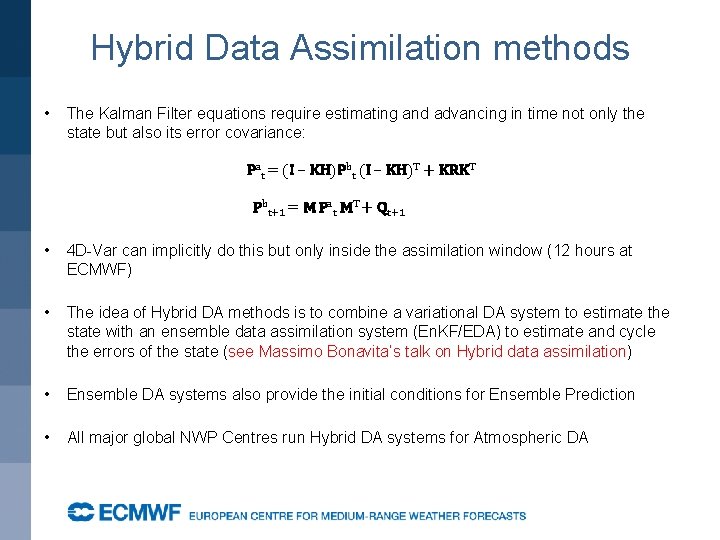
Hybrid Data Assimilation methods • The Kalman Filter equations require estimating and advancing in time not only the state but also its error covariance: Pat = (I – KH)Pbt (I – KH)T + KRKT Pbt+1 = M Pat MT + Qt+1 • 4 D-Var can implicitly do this but only inside the assimilation window (12 hours at ECMWF) • The idea of Hybrid DA methods is to combine a variational DA system to estimate the state with an ensemble data assimilation system (En. KF/EDA) to estimate and cycle the errors of the state (see Massimo Bonavita’s talk on Hybrid data assimilation) • Ensemble DA systems also provide the initial conditions for Ensemble Prediction • All major global NWP Centres run Hybrid DA systems for Atmospheric DA

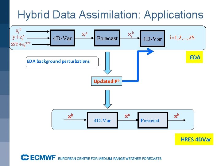
Hybrid Data Assimilation: Applications xib y+εio 4 D-Var xia Forecast xib SST+εi. SST 4 D-Var i=1, 2, …, 25 EDA background perturbations Updated Pb xb 4 D-Var xa Forecast xb HRES 4 DVar

Earth System Data Assimilation • We have discussed Data Assimilation methods with an emphasis on global Atmospheric NWP applications • The DA methods presented are however general: which one to apply to a given problem depends on the characteristics of the problem (size of the state vector, number and quality of observations, available computing resources, available manpower, …) • You have seen applications in Atmospheric Composition DA (4 D-Var: Antje Inness’s talk); in Ocean Data Assimilation (3 D-Var FGAT: Hao Zuo’s talk); in Land Data Assimilation (O. I. , Simplified Extended KF: Patricia de Rosnay’s talk) • In current ECMWF DA the Earth system’s components are at most only weakly coupled (through a coupled model background forecast) • Phil Browne’s talk has given you a sense of some of the challenges and the potential benefits of a stronger coupling in the data assimilation for the different components of the Earth System

Earth System Data Assimilation • We have discussed Data Assimilation methods for the Earth System with an emphasis on producing the best initial state estimate forecasting at short, extended and even seasonal timescales • An increasingly important application of Earth System DA is to help to reconstruct the past climate and weather (see Patrick Laloyaux’s talk on Reanalysis methods) • As DA methods have dramatically improved over the years we are able to make better use of past observational records and more robustly estimate climatic trends

Earth System DA: Challenges • We have tried to provide you with a description of the state of the art in data assimilation methods for Earth System applications • As you have gathered from the various talks a number of challenges lie ahead • We would like to highlight a few of the more exciting: a) All current methods rely implicitly or explicitly on an assumption of Gaussian errors and quasi-linear error evolution: can we go beyond it? b) Coupling among the different Earth System components is weak in data assimilation: what are the best ways towards a strong coupling approach? c) Volume of observations (especially satellite derived) keeps on increasing at a very fast rate: Are our current DA methods able to make good use of all these data? d) ….

Thank you for being such an attentive audience!