Data assimilation schemes in numerical weather forecasting and

Data assimilation schemes in numerical weather forecasting and their link with ensemble forecasting Gérald Desroziers Météo-France, Toulouse, France

Outline § Numerical weather prediction § Data assimilation § A posteriori diagnostics: optimizing error statistics § Ensemble assimilation § Impact of observations on analyses and forecasts § Conclusion and perspectives

Outline § Numerical weather prediction § Data assimilation § A posteriori diagnostics: optimizing error statistics § Ensemble assimilation § Impact of observations on analyses and forecasts § Conclusion and perspectives

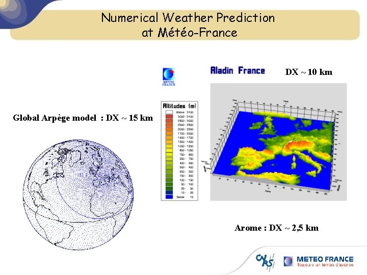
Numerical Weather Prediction at Météo-France DX ~ 10 km Global Arpège model : DX ~ 15 km Arome : DX ~ 2, 5 km

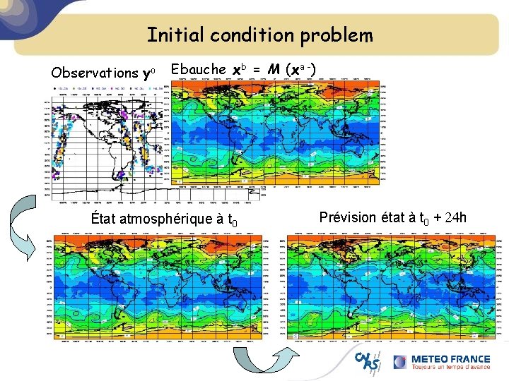
Initial condition problem Observations yo Ebauche xb = M (xa -) État atmosphérique à t 0 Prévision état à t 0 + 24 h

Outline § Numerical weather prediction § Data assimilation § A posteriori diagnostics: optimizing error statistics § Ensemble assimilation § Impact of observations on analyses and forecasts § Conclusion and perspectives

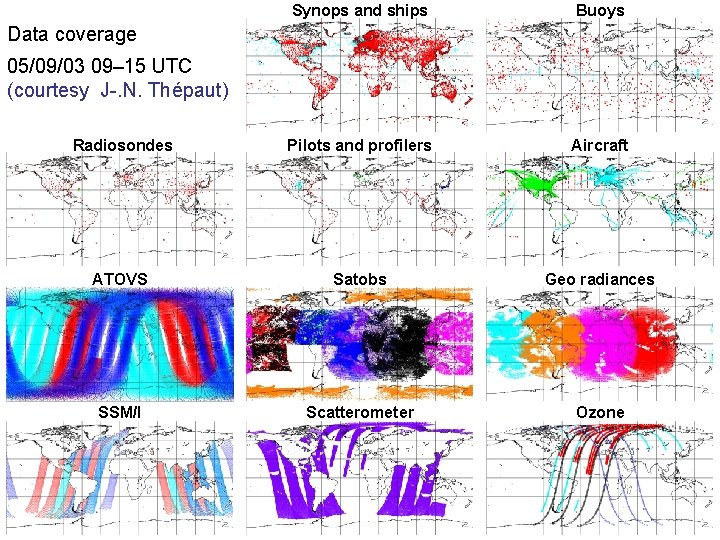
Synops and ships Buoys Radiosondes Pilots and profilers Aircraft ATOVS Satobs Geo radiances SSM/I Scatterometer Ozone Data coverage 05/09/03 09– 15 UTC (courtesy J-. N. Thépaut)

Satellites (EUMETSAT)

Satellite data sources (courtesy J-. N. Thépaut, ECMWF)

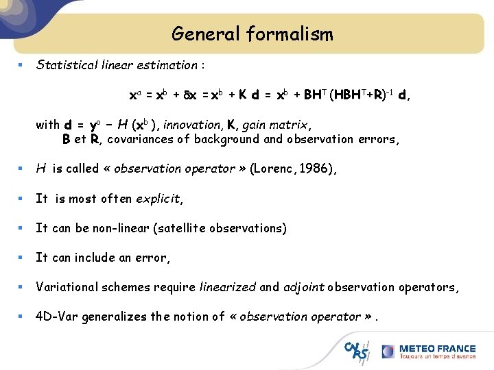
General formalism § Statistical linear estimation : xa = xb + dx = xb + K d = xb + BHT (HBHT+R)-1 d, with d = yo – H (xb ), innovation, K, gain matrix, B et R, covariances of background and observation errors, § H is called « observation operator » (Lorenc, 1986), § It is most often explicit, § It can be non-linear (satellite observations) § It can include an error, § Variational schemes require linearized and adjoint observation operators, § 4 D-Var generalizes the notion of « observation operator » .

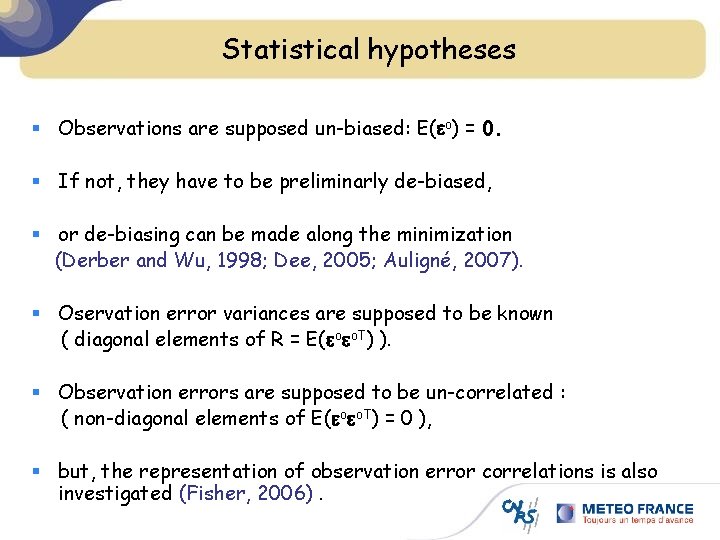
Statistical hypotheses § Observations are supposed un-biased: E(eo) = 0. § If not, they have to be preliminarly de-biased, § or de-biasing can be made along the minimization (Derber and Wu, 1998; Dee, 2005; Auligné, 2007). § Oservation error variances are supposed to be known ( diagonal elements of R = E(eoeo. T) ). § Observation errors are supposed to be un-correlated : ( non-diagonal elements of E(eoeo. T) = 0 ), § but, the representation of observation error correlations is also investigated (Fisher, 2006).

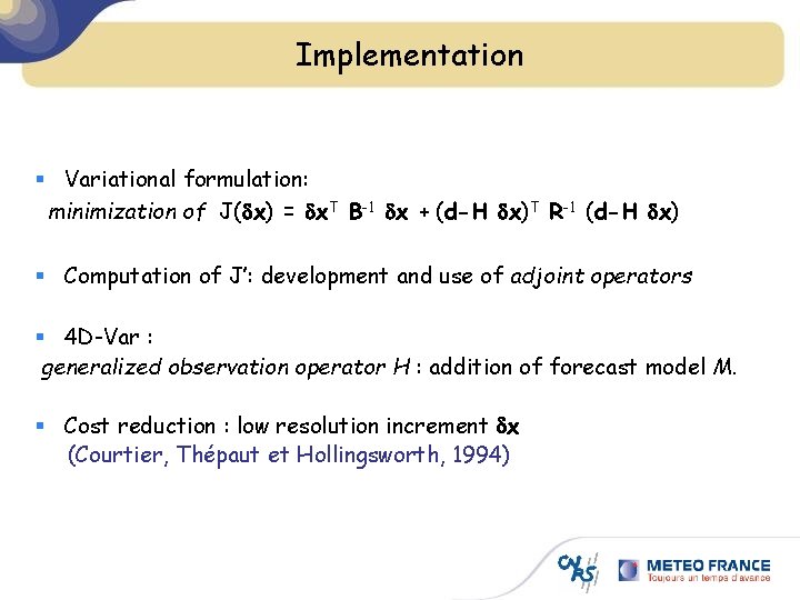
Implementation § Variational formulation: minimization of J(dx) = dx. T B-1 dx + (d-H dx)T R-1 (d-H dx) § Computation of J’: development and use of adjoint operators § 4 D-Var : generalized observation operator H : addition of forecast model M. § Cost reduction : low resolution increment dx (Courtier, Thépaut et Hollingsworth, 1994)

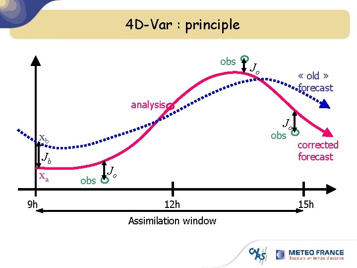
4 D-Var : principle obs Jo « old » forecast analysis Jo obs xb Jb xa 9 h obs corrected forecast Jo 12 h Assimilation window 15 h

Outline § Numerical weather prediction § Data assimilation § A posteriori diagnostics: optimizing error statistics § Ensemble assimilation § Impact of observations on analyses and forecasts § Conclusion and perspectives

A posteriori diagnostics § Is the system consistent? § We should have § but also E[J(xa) ] = p, p = total number of observations, E[Joi(xa) ] = pi – Tr(Ri-1/2 H i A H i. T Ri-1/2 ), pi : number of observations associated with Joi (Talagrand, 1999). § Computation of optimal E[Joi(xa) ] by a Monte-Carlo procedure is possible. (Desroziers et Ivanov, 2001).

Application : optimisation of R ∙ ∙ ∙ ∙ ∙ E[Joi (xa)] = (E[Joi (xa)])opt. ∙ ∙ ∙ One tries to obtain by adjusting the soi Optimisation of HIRS ∙ ∙∙ (Chapnik, et al, 2004; Buehner, 2005) so

Outline § Numerical weather prediction § Data assimilation § A posteriori diagnostics: optimizing error statistics § Ensemble assimilation § Impact of observations on analyses and forecasts § Conclusion and perspectives

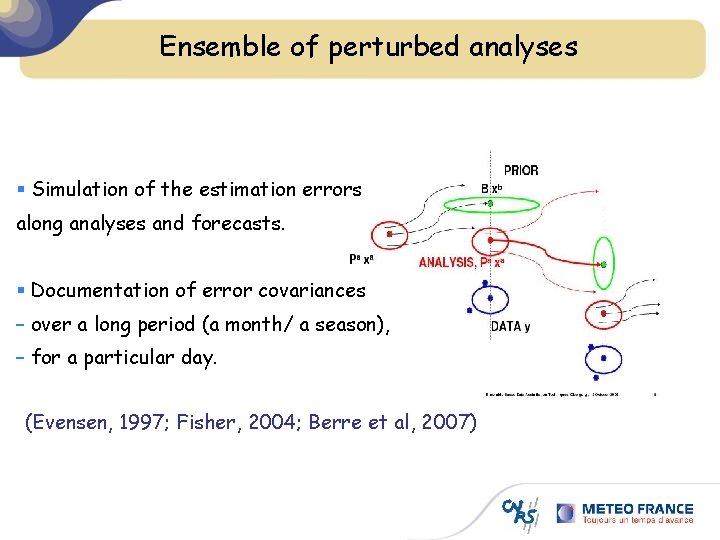
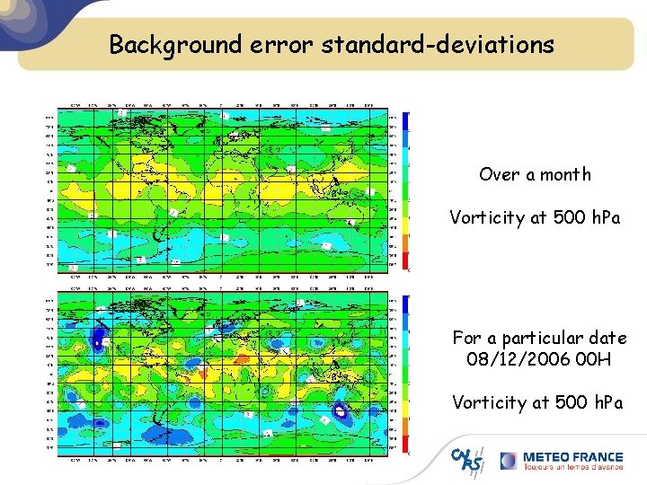
Ensemble of perturbed analyses § Simulation of the estimation errors along analyses and forecasts. § Documentation of error covariances – over a long period (a month/ a season), – for a particular day. (Evensen, 1997; Fisher, 2004; Berre et al, 2007)

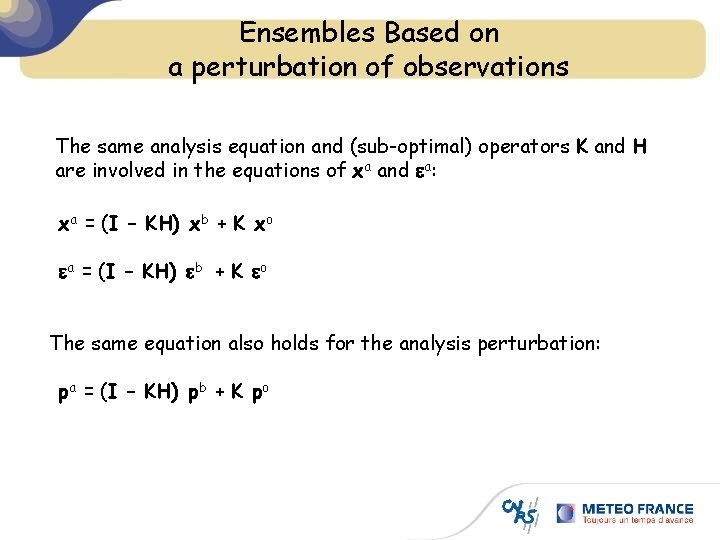
Ensembles Based on a perturbation of observations The same analysis equation and (sub-optimal) operators K and H are involved in the equations of xa and ea: xa = (I – KH) xb + K xo ea = (I – KH) eb + K eo The same equation also holds for the analysis perturbation: pa = (I – KH) pb + K po

Background error standard-deviations Over a month Vorticity at 500 h. Pa For a particular date 08/12/2006 00 H Vorticity at 500 h. Pa

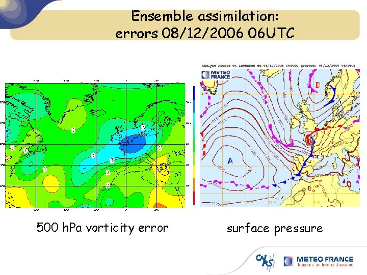
Ensemble assimilation: errors 08/12/2006 06 UTC 500 h. Pa vorticity error surface pressure

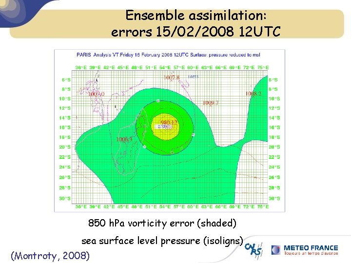
Ensemble assimilation: errors 15/02/2008 12 UTC 850 h. Pa vorticity error (shaded) sea surface level pressure (isoligns) (Montroty, 2008)

Outline § Numerical weather prediction § Data assimilation § A posteriori diagnostics: optimizing error statistics § Ensemble assimilation § Impact of observations on analyses and forecasts § Conclusion and perspectives

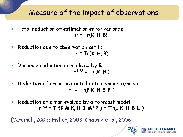
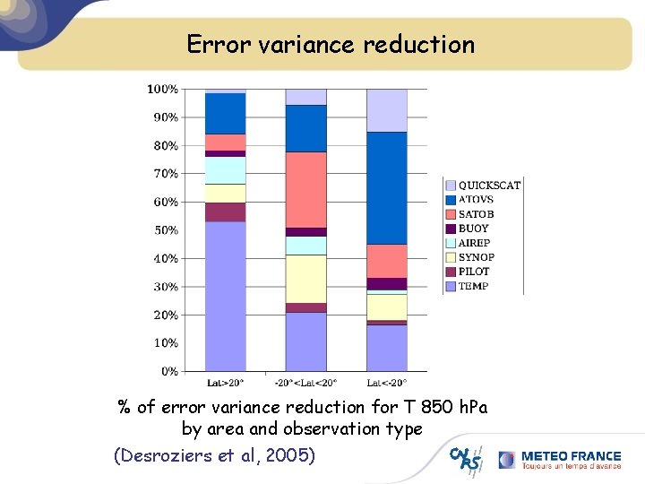
Measure of the impact of observations § Total reduction of estimation error variance: r = Tr(K H B) § Reduction due to observation set i : ri = Tr(Ki Hi B) § Variance reduction normalized by B : ri. DFS = Tr(Ki Hi) § Reduction of error projected onto a variable/area: ri. P = Tr(P Ki Hi B PT) § Reduction of error evolved by a forecast model: ri. PM = Tr(P M Ki Hi B MT PT) = Tr(L Ki Hi B LT) (Cardinali, 2003; Fisher, 2003; Chapnik et al, 2006)

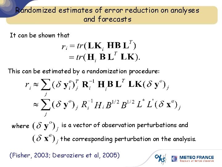
Randomized estimates of error reduction on analyses and forecasts It can be shown that This can be estimated by a randomization procedure: where is a vector of observation perturbations and the corresponding perturbation on the analysis. (Fisher, 2003; Desroziers et al, 2005)

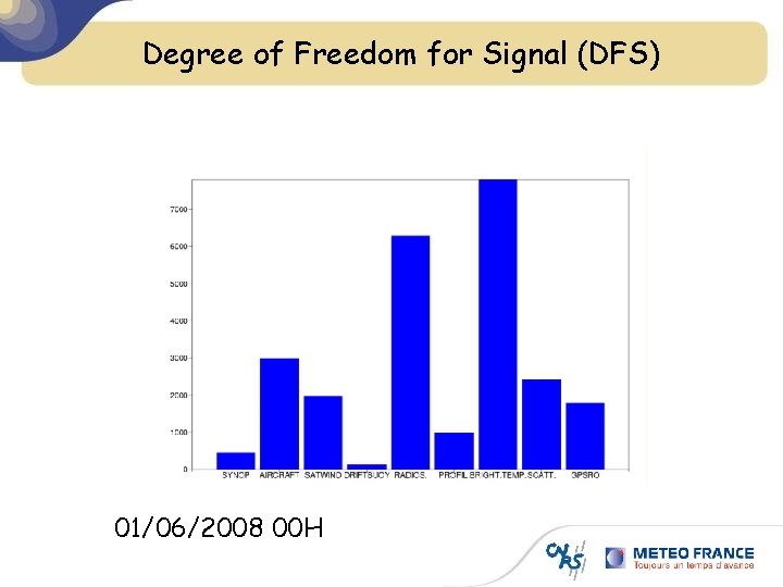
Degree of Freedom for Signal (DFS) 01/06/2008 00 H

Error variance reduction % of error variance reduction for T 850 h. Pa by area and observation type (Desroziers et al, 2005)

Outline § Numerical weather prediction § Data assimilation § A posteriori diagnostics: optimizing error statistics § Ensemble assimilation § Impact of observations on analyses and forecasts § Conclusion and perspectives

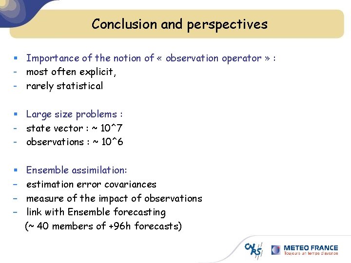
Conclusion and perspectives § Importance of the notion of « observation operator » : - most often explicit, - rarely statistical § Large size problems : - state vector : ~ 10^7 - observations : ~ 10^6 § – – – Ensemble assimilation: estimation error covariances measure of the impact of observations link with Ensemble forecasting (~ 40 members of +96 h forecasts)