Data Assimilation in Meteorology Chris Budd Joint work

Data Assimilation in Meteorology Chris Budd Joint work with Chiara Piccolo, Mike Cullen (Met Office) Melina Freitag, Phil Browne, Emily Walsh, Nathan Smith and Sian Jenkins (Bath)

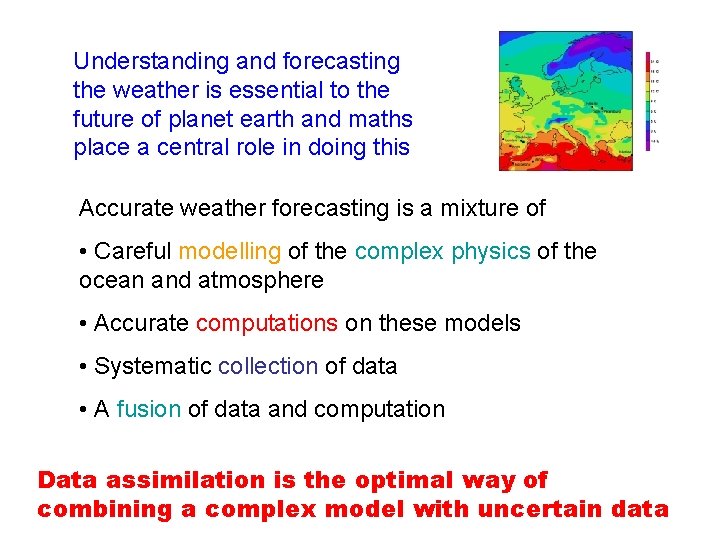
Understanding and forecasting the weather is essential to the future of planet earth and maths place a central role in doing this Accurate weather forecasting is a mixture of • Careful modelling of the complex physics of the ocean and atmosphere • Accurate computations on these models • Systematic collection of data • A fusion of data and computation Data assimilation is the optimal way of combining a complex model with uncertain data

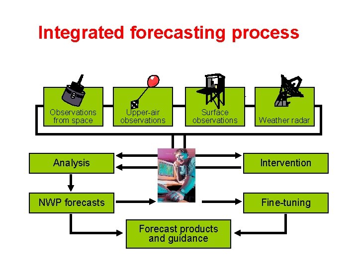
Integrated forecasting process Observations from space Upper-air observations Surface observations Weather radar Analysis Intervention NWP forecasts Fine-tuning Forecast products and guidance

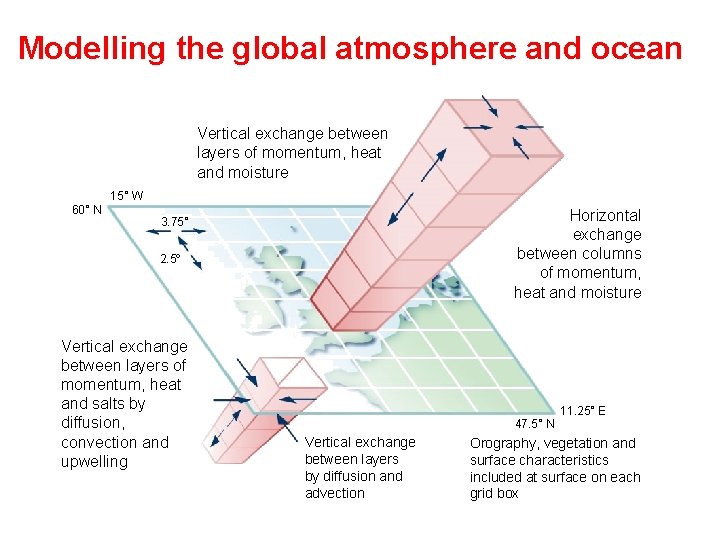
Modelling the global atmosphere and ocean Vertical exchange between layers of momentum, heat and moisture 15° W 60° N Horizontal exchange between columns of momentum, heat and moisture 3. 75° 2. 5° Vertical exchange between layers of momentum, heat and salts by diffusion, convection and upwelling 47. 5° N Vertical exchange between layers by diffusion and advection 11. 25° E Orography, vegetation and surface characteristics included at surface on each grid box

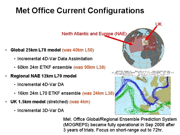
Met Office Current Configurations UK North Atlantic and Europe (NAE) • Global 25 km L 70 model (was 40 km L 50) • Incremental 4 D-Var Data Assimilation • 60 km 24 m ETKF ensemble (was 90 km L 38) • Regional NAE 12 km L 70 model • Incremental 4 D-Var DA • 16 km 24 m L 70 ETKF ensemble (was 24 km L 38) • UK 1. 5 km model (stretched) (was 4 km) • Incremental 3 D-Var DA Met. Office Global/Regional Ensemble Prediction System (MOGREPS) became fully operational in Sep 2008 after 3 years of trials. Focus on short-range out to 72 hr.

Data: Sources of observation

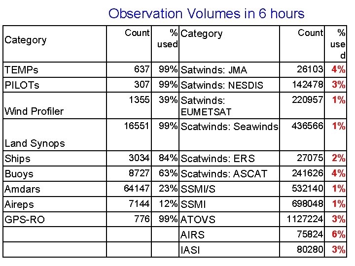
Observation Volumes in 6 hours Category TEMPs PILOTs Wind Profiler Land Synops Ships Buoys Amdars Aireps GPS-RO Count % Category used 637 99% Satwinds: JMA Count % use d 26103 4% 307 99% Satwinds: NESDIS 142478 3% 1355 39% Satwinds: EUMETSAT 16551 99% Scatwinds: Seawinds 220957 1% 3034 84% Scatwinds: ERS 8727 63% Scatwinds: ASCAT 436566 1% 27075 2% 241626 4% 64147 23% SSMI/S 532140 1% 7144 12% SSMI 698048 1% 776 99% ATOVS AIRS IASI 1127224 3% 75824 6% 80280 3%

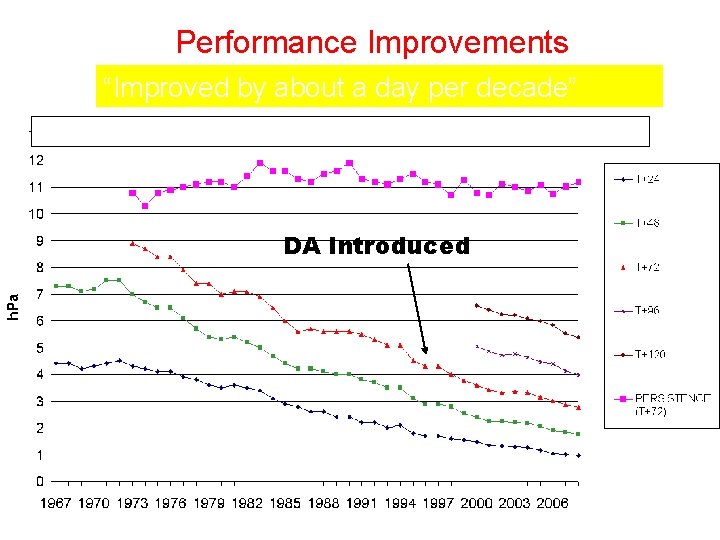
Performance Improvements “Improved by about a day per decade” Met Office RMS surface pressure error over the N. Atlantic & W. Europe DA Introduced Andrew Lorenc

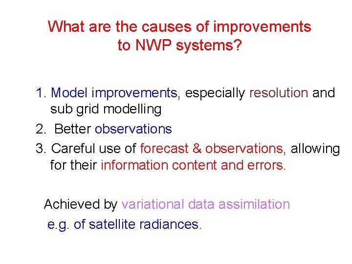
What are the causes of improvements to NWP systems? 1. Model improvements, especially resolution and sub grid modelling 2. Better observations 3. Careful use of forecast & observations, allowing for their information content and errors. Achieved by variational data assimilation e. g. of satellite radiances.

Basic Idea of Data Assimilation True state of the weather is Numerical Weather Prediction NWP calculation gives a predicted state with an error Make a series of observations y of some function of the true state Eg. Limited set of temperature measurements with error Now combine the prediction with the observations

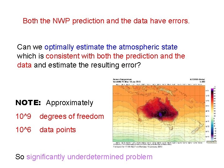
Both the NWP prediction and the data have errors. Can we optimally estimate the atmospheric state which is consistent with both the prediction and the data and estimate the resulting error? NOTE: Approximately 10^9 degrees of freedom 10^6 data points So significantly underdetermined problem

Best state estimate Data y analysis NWP prediction Assume initially: Use to produce forecast 6 hours later 1. Errors are unbiased Gaussian variables 2. Data and NWP prediction errors are uncorrelated 3. H(x) is a linear operator

Can estimate using Bayesian analyis: Maximum likelihood estimate of data y given Posterior Prior Likelihood Best RMS unbiased estimate of the true state: BLUE Minimum error variance

Assumptions about the error Data error: Gaussian, Covariance R Background (NWP) error: Gaussian, Covariance B BLUE: NOTE: Find which minimises

If R and B are known the best estimate of the analysis is Covariance of the analysis error Kalman filter: Continuously updates the forecast and its error given the incoming data.

Implementation: In the context of minimising the functional This is implemented as 3 D-VAR (since 1999 in the Met Office) : Background, derived from 6 hour NWP forecast : Analysis : NWP forecast using as initial data

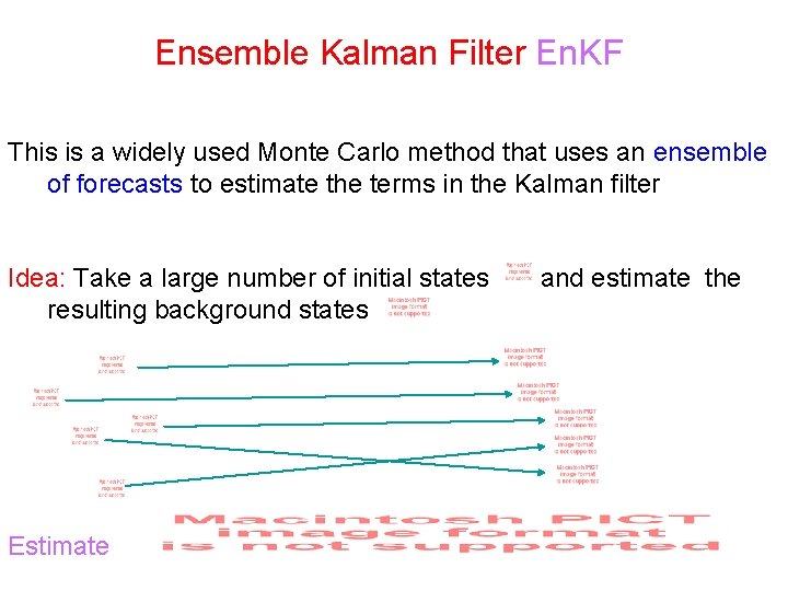
Ensemble Kalman Filter En. KF This is a widely used Monte Carlo method that uses an ensemble of forecasts to estimate the terms in the Kalman filter Idea: Take a large number of initial states resulting background states Estimate and estimate the

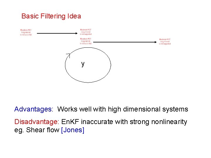
Basic Filtering Idea y Advantages: Works well with high dimensional systems Disadvantage: En. KF inaccurate with strong nonlinearity eg. Shear flow [Jones]

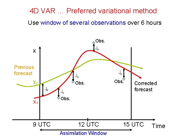
4 D VAR … Preferred variational method Use window of several observations over 6 hours Obs. Jo x Previous forecast Jo xb Obs. Jb xa 9 UTC Jo Jo Obs. Corrected forecast Obs. 12 UTC Assimilation Window 15 UTC Time

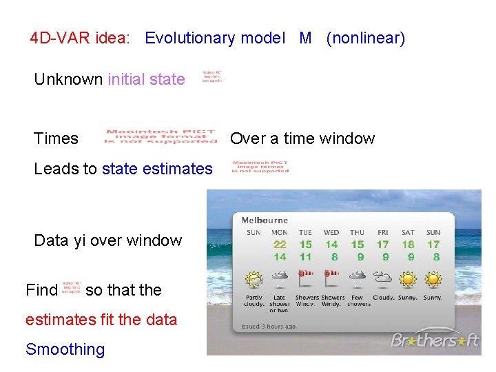
4 D-VAR idea: Evolutionary model M (nonlinear) Unknown initial state Times Over a time window Leads to state estimates Data yi over window Find so that the estimates fit the data Smoothing

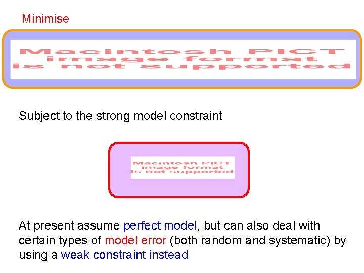
Minimise Subject to the strong model constraint At present assume perfect model, but can also deal with certain types of model error (both random and systematic) by using a weak constraint instead

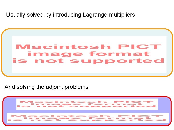
Usually solved by introducing Lagrange multipliers And solving the adjoint problems

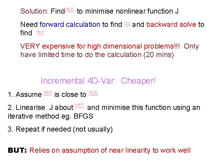
Solution: Find to minimise nonlinear function J Need forward calculation to find and backward solve to VERY expensive for high dimensional problems!!! Only have limited time to do the calculation (20 mins) Incremental 4 D-Var: Cheaper! 1. Assume is close to 2. Linearise J about and minimise this function using an iterative method eg. BFGS 3. Repeat if needed (not usually) BUT: Relies on assumption of near linearity to work well

Very effective method!! Met Office operational in 2004 [Lorenc, …. ] Used by many other centres

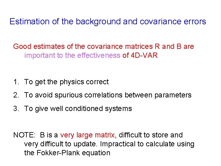
Estimation of the background and covariance errors Good estimates of the covariance matrices R and B are important to the effectiveness of 4 D-VAR 1. To get the physics correct 2. To avoid spurious correlations between parameters 3. To give well conditioned systems NOTE: B is a very large matrix, difficult to store and very difficult to update. Impractical to calculate using the Fokker-Plank equation

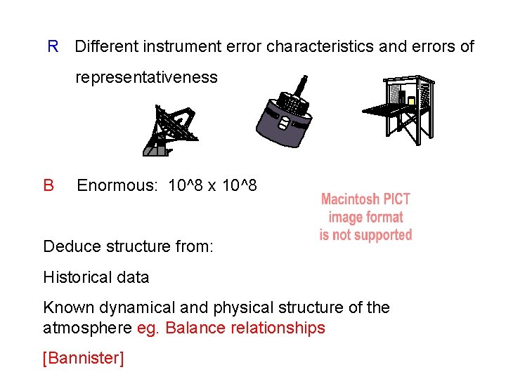
R Different instrument error characteristics and errors of representativeness B Enormous: 10^8 x 10^8 Deduce structure from: Historical data Known dynamical and physical structure of the atmosphere eg. Balance relationships [Bannister]

Build meteorology into the calculation of B through Control Variable Transformations (CVTs) IDEA: Choose more ‘natural’ physical variables which have uncorrelated errors so that the transformed covariance matrix is block diagonal or even the identity Set Reduces the complexity of the system AND gives better conditioning for the linear systems

Separates physical parameters into uncorrelated ones eg. temperature, wind, balanced and unbalanced Reduces vertical correlations by projecting onto empirical orthogonal vertical modes Reduces horizontal correlations by projecting onto spherical harmonics Effective, but errors arise due to lack of resolution of physical features leading to spurious correlations.

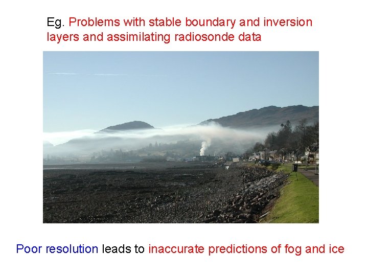
Eg. Problems with stable boundary and inversion layers and assimilating radiosonde data Poor resolution leads to inaccurate predictions of fog and ice

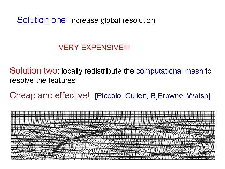
Solution one: increase global resolution VERY EXPENSIVE!!! Solution two: locally redistribute the computational mesh to resolve the features Cheap and effective! [Piccolo, Cullen, B, Browne, Walsh]

Adjust the vertical coordinates to concentrate points close to the inversion layer and reduce correlations Introduce an extra transformation Adaptive mesh transformation applied to latitude-longitude coordinates

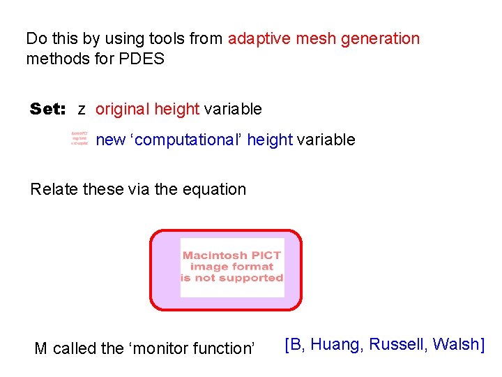
Do this by using tools from adaptive mesh generation methods for PDES Set: z original height variable new ‘computational’ height variable Relate these via the equation M called the ‘monitor function’ [B, Huang, Russell, Walsh]

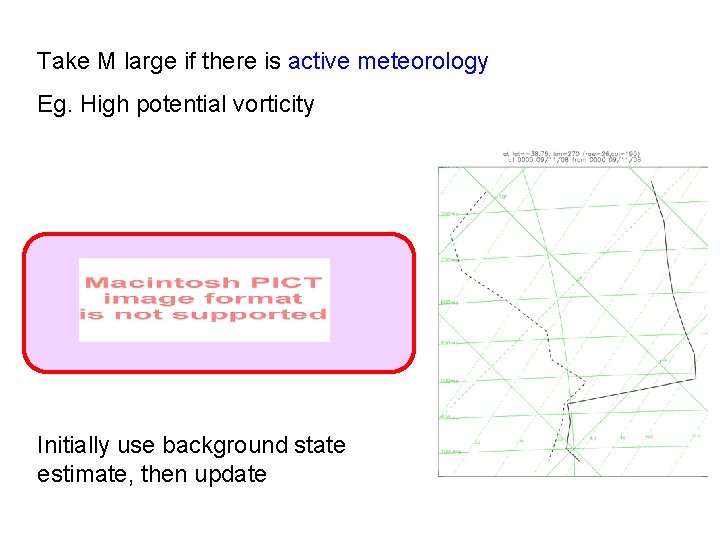
Take M large if there is active meteorology Eg. High potential vorticity Initially use background state estimate, then update

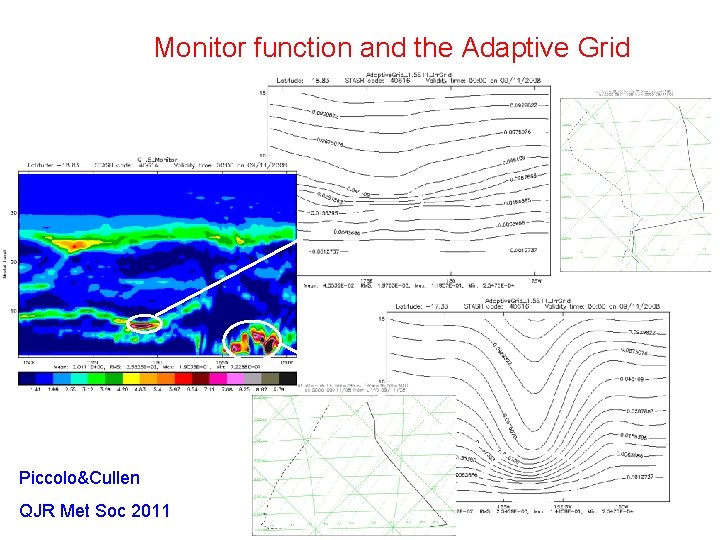
Monitor function and the Adaptive Grid Piccolo&Cullen QJR Met Soc 2011 © Crown copyright Met Office

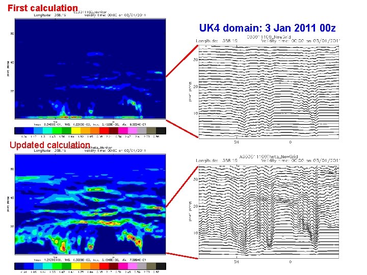
First calculation UK 4 domain: 3 Jan 2011 00 z Updated calculation © Crown copyright Met Office

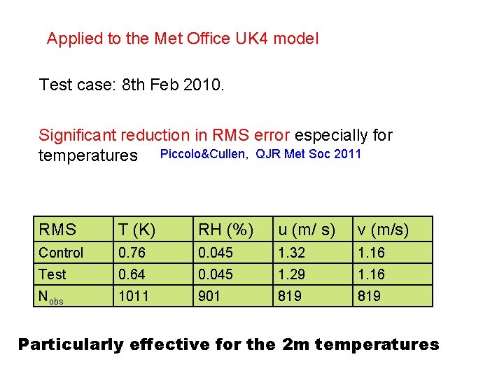
Applied to the Met Office UK 4 model Test case: 8 th Feb 2010. Significant reduction in RMS error especially for temperatures Piccolo&Cullen, QJR Met Soc 2011 RMS T (K) RH (%) u (m/ s) v (m/s) Control 0. 76 0. 045 1. 32 1. 16 Test 0. 64 0. 045 1. 29 1. 16 Nobs 1011 901 819 Particularly effective for the 2 m temperatures

Used together with Met Office Open Road software to advise councils on road gritting over Christmas

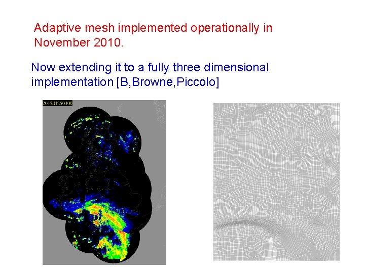
Adaptive mesh implemented operationally in November 2010. Now extending it to a fully three dimensional implementation [B, Browne, Piccolo]

Other refinements to 4 D-Var Change in the background norm [Freitag, B, Nichols] Total variation: Gives significantly better resolution of fronts, shocks and other localised features But. . Hard to implement in high dimensions!!

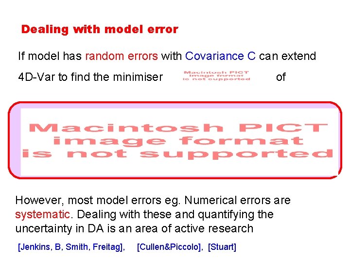
Dealing with model error If model has random errors with Covariance C can extend 4 D-Var to find the minimiser of However, most model errors eg. Numerical errors are systematic. Dealing with these and quantifying the uncertainty in DA is an area of active research [Jenkins, B, Smith, Freitag], [Cullen&Piccolo], [Stuart]

Dealing with nonlinearity Lot of research into finding a compromise between dealing with the high dimensionality and nonlinearity in the system Better use of appropriate (eg. Lagrangian) data Tuning method to data [Jones, Stuart, Apte] Use of particle filters and MCMC methods [Peter Van Leeuwan]

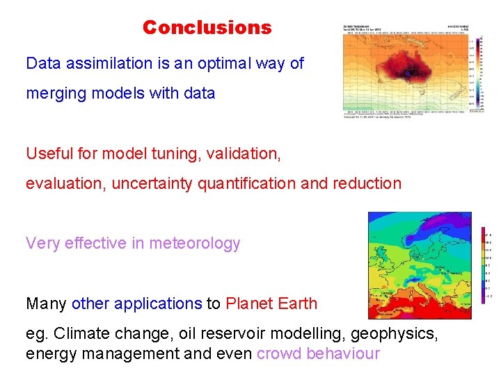
Conclusions Data assimilation is an optimal way of merging models with data Useful for model tuning, validation, evaluation, uncertainty quantification and reduction Very effective in meteorology Many other applications to Planet Earth eg. Climate change, oil reservoir modelling, geophysics, energy management and even crowd behaviour

Problems with the simple Kalman Filter • Assumption of Gaussian random variables • Assumption of linearity • Assumption of known covariances • Covariance matrix B is VERY large for meteorological problems • Minimisation is a large complex problem

Problems with 4 D Var Accuracy • Estimation of the background covariance matrix • Ill conditioning of the linear systems • Reliance of near linearity • Inappropriate use of background data • Incorrect covariance between data • Unresolved random and systematic model error • Poor resolution in the model Improvements subject to much research