Data Assimilation for NWP 4 Evaluation and improving

Data Assimilation for NWP 4. Evaluation and improving use of observations Andrew Lorenc www. metoffice. gov. uk © Crown Copyright 2017, Met Office

Estimating Covariances R B Q © Crown copyright Met Office Andrew Lorenc 2

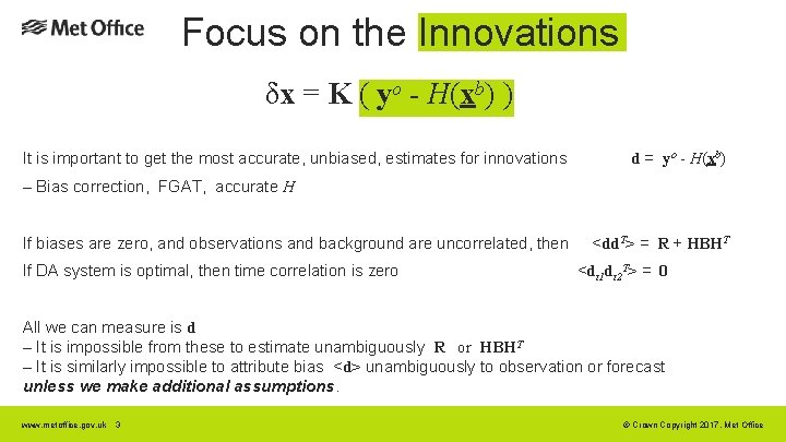
Focus on the Innovations δx = K ( yo - H(xb) ) It is important to get the most accurate, unbiased, estimates for innovations d = yo - H(xb) – Bias correction, FGAT, accurate H If biases are zero, and observations and background are uncorrelated, then If DA system is optimal, then time correlation is zero <dd. T> = R + HBHT <dt 1 dt 2 T> = 0 All we can measure is d – It is impossible from these to estimate unambiguously R or HBHT – It is similarly impossible to attribute bias <d> unambiguously to observation or forecast unless we make additional assumptions. www. metoffice. gov. uk 3 © Crown Copyright 2017, Met Office

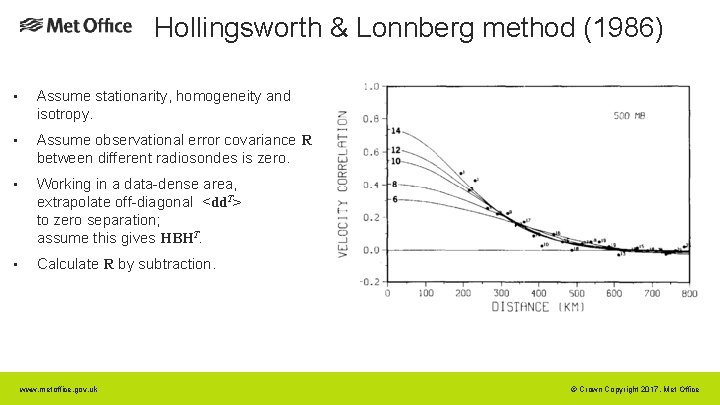
Hollingsworth & Lonnberg method (1986) • Assume stationarity, homogeneity and isotropy. • Assume observational error covariance R between different radiosondes is zero. • Working in a data-dense area, extrapolate off-diagonal <dd. T> to zero separation; assume this gives HBHT. • Calculate R by subtraction. www. metoffice. gov. uk © Crown Copyright 2017, Met Office

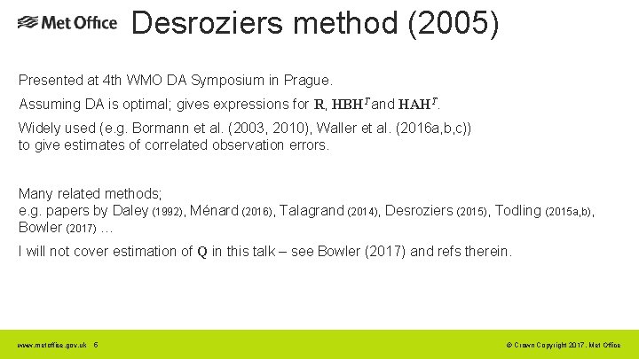
Desroziers method (2005) Presented at 4 th WMO DA Symposium in Prague. Assuming DA is optimal; gives expressions for R, HBHT and HAHT. Widely used (e. g. Bormann et al. (2003, 2010), Waller et al. (2016 a, b, c)) to give estimates of correlated observation errors. Many related methods; e. g. papers by Daley (1992), Ménard (2016), Talagrand (2014), Desroziers (2015), Todling (2015 a, b), Bowler (2017) … I will not cover estimation of Q in this talk – see Bowler (2017) and refs therein. www. metoffice. gov. uk 5 © Crown Copyright 2017, Met Office

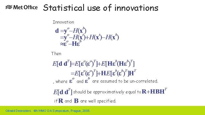
Statistical use of innovations Innovation Then , where and are assumed to be un-correlated. should be approximatively equal to if and are well specified. Gérald Desroziers. 4 th WMO DA Symposium, Prague, 2005.

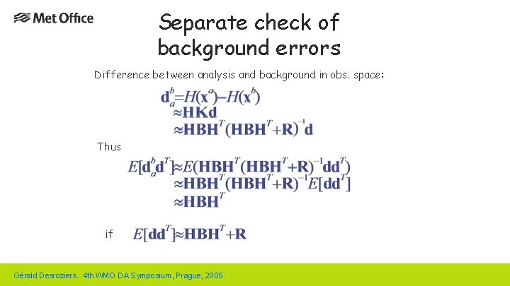
Separate check of background errors Difference between analysis and background in obs. space: Thus if Gérald Desroziers. 4 th WMO DA Symposium, Prague, 2005.

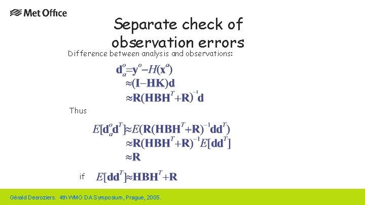
Separate check of observation errors Difference between analysis and observations: Thus if Gérald Desroziers. 4 th WMO DA Symposium, Prague, 2005.

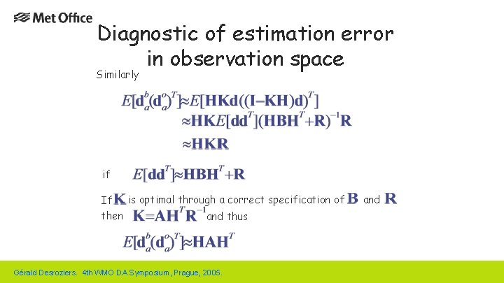
Diagnostic of estimation error in observation space Similarly if If is optimal through a correct specification of then and thus Gérald Desroziers. 4 th WMO DA Symposium, Prague, 2005. and

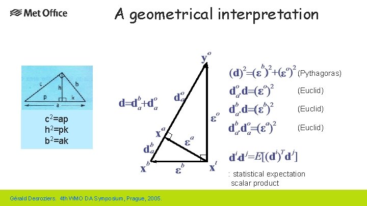
A geometrical interpretation (Pythagoras) (Euclid) c 2=ap h 2=pk b 2=ak (Euclid) : statistical expectation scalar product Gérald Desroziers. 4 th WMO DA Symposium, Prague, 2005.

Variational Bias Correction Var. BC © Crown copyright Met Office Andrew Lorenc 11

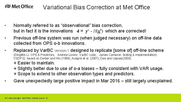
Variational Bias Correction at Met Office • Normally referred to as “observational” bias correction, but in fact it is the innovations d = yo - H(xb) which are corrected! • Previous off-line system was run (when judged necessary) on off-line data collected from OPS o-b innovations. • Replaced by Var. BC version-1 designed to replicate [some of] off-line scheme (Ding. Min Li: OPS & Predictors, Andrew Lorenc: Var. BC code, James Cameron: testing & implementation) VSDP 32: based on Derber and Wu (1998), Auligné et al. (2007), Dee and Uppala(2009). + Easier to maintain. + Slightly better due to use of o-a biases – fully consistent with VAR usage. + Scope to extend to other observation types and predictors. • Gave unexpectedly large positive impact in Mar 2016 – still largely unexplained. © Crown copyright Met Office Andrew Lorenc 12

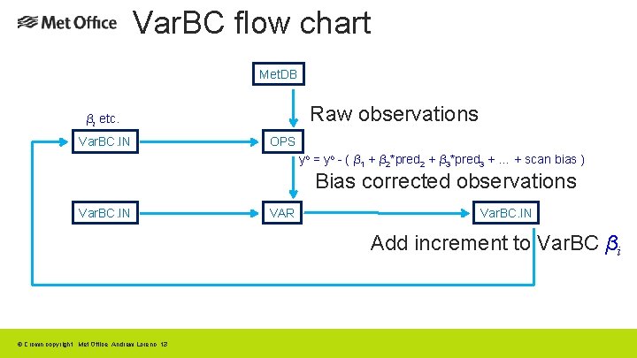
Var. BC flow chart Met. DB Raw observations βi etc. Var. BC. IN OPS yo = yo - ( β 1 + β 2*pred 2 + β 3*pred 3 + … + scan bias ) Bias corrected observations Var. BC. IN VAR Var. BC. IN Add increment to Var. BC βi © Crown copyright Met Office Andrew Lorenc 13

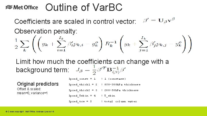
Outline of Var. BC Coefficients are scaled in control vector: Observation penalty: Limit how much the coefficients can change with a background term: Ipred_const = 1 ! 1 (constant) Original predictors Ipred_thick 1 = 2 ! 850 -300 h. Pa thickness Offset & scaled: mean≈0, variance≈1 Ipred_thick 2 = 3 ! 200 -50 h. Pa thickness Ipred_Tskin = 4 ! T_skin Ipred_tcw = 5 ! total column water © Crown copyright Met Office Andrew Lorenc 14

Quality Control Station lists, Bayesian in OPS, Var. QC © Crown copyright Met Office Andrew Lorenc 15

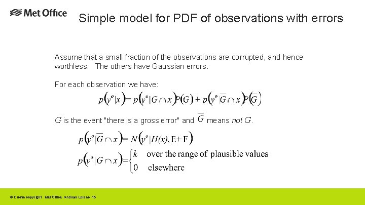
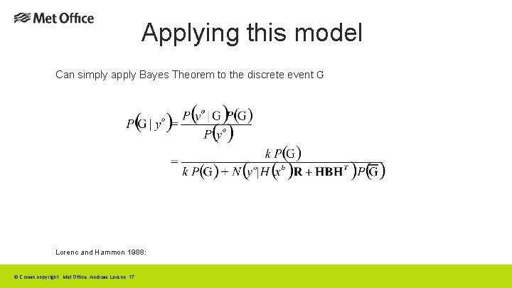
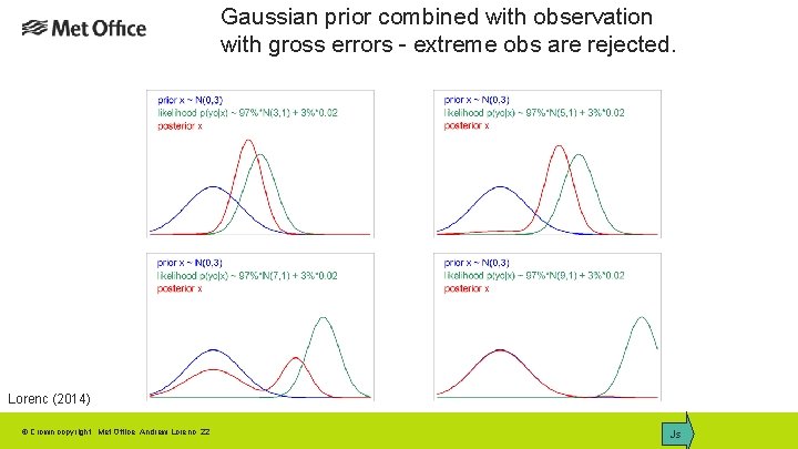
Simple model for PDF of observations with errors Assume that a small fraction of the observations are corrupted, and hence worthless. The others have Gaussian errors. For each observation we have: G is the event "there is a gross error" and © Crown copyright Met Office Andrew Lorenc 16 means not G.

Applying this model Can simply apply Bayes Theorem to the discrete event G Lorenc and Hammon 1988: © Crown copyright Met Office Andrew Lorenc 17

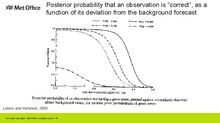
Posterior probability that an observation is “correct”, as a function of its deviation from the background forecast Lorenc and Hammon, 1988 © Crown copyright Met Office Andrew Lorenc 18

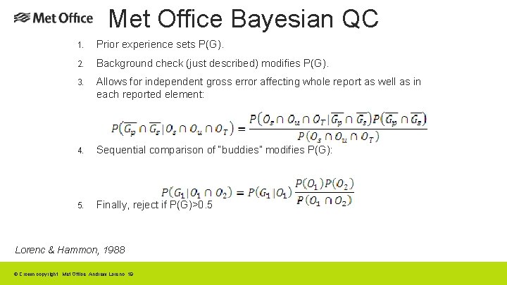
Met Office Bayesian QC 1. Prior experience sets P(G). 2. Background check (just described) modifies P(G). 3. Allows for independent gross error affecting whole report as well as in each reported element: 4. Sequential comparison of “buddies” modifies P(G): 5. Finally, reject if P(G)>0. 5 Lorenc & Hammon, 1988 © Crown copyright Met Office Andrew Lorenc 19

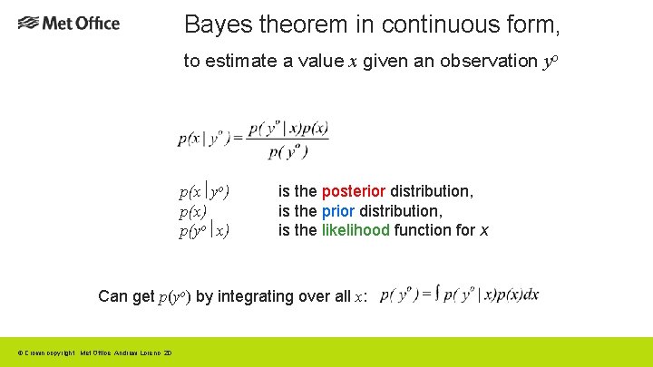
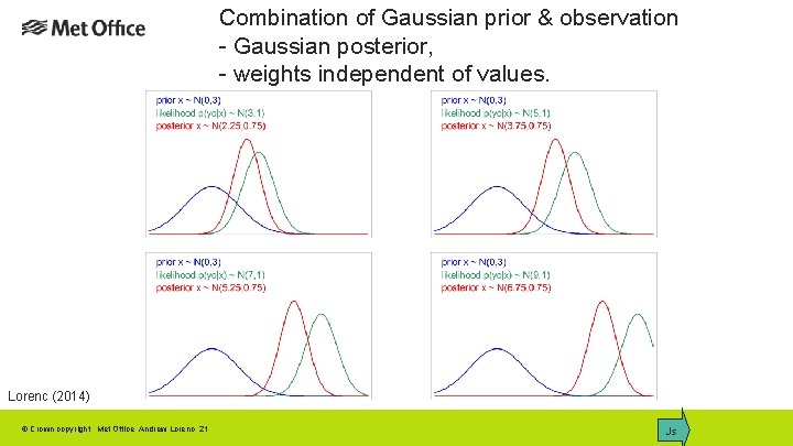
Bayes theorem in continuous form, to estimate a value x given an observation yo p(x yo) p(x) p(yo x) is the posterior distribution, is the prior distribution, is the likelihood function for x Can get p(yo) by integrating over all x: © Crown copyright Met Office Andrew Lorenc 20

Combination of Gaussian prior & observation - Gaussian posterior, - weights independent of values. Lorenc (2014) © Crown copyright Met Office Andrew Lorenc 21 Js

Gaussian prior combined with observation with gross errors - extreme obs are rejected. Lorenc (2014) © Crown copyright Met Office Andrew Lorenc 22 Js

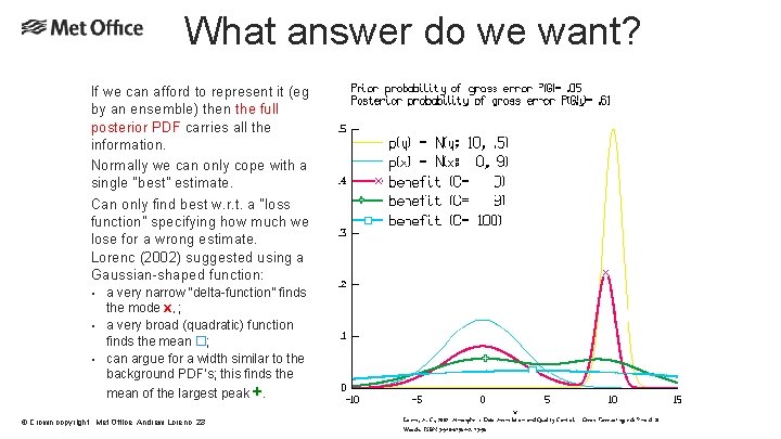
What answer do we want? If we can afford to represent it (eg by an ensemble) then the full posterior PDF carries all the information. Normally we can only cope with a single “best” estimate. Can only find best w. r. t. a “loss function” specifying how much we lose for a wrong estimate. Lorenc (2002) suggested using a Gaussian-shaped function: • • • a very narrow “delta-function” finds the mode X, ; a very broad (quadratic) function finds the mean ; can argue for a width similar to the background PDF’s; this finds the mean of the largest peak +. © Crown copyright Met Office Andrew Lorenc 23 Lorenc, A. C. , 2002: Atmospheric Data Assimilation and Quality Control. Ocean Forecasting , eds Pinardi & Woods. ISBN 3 -540 -67964 -2. 73 -96

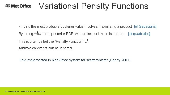
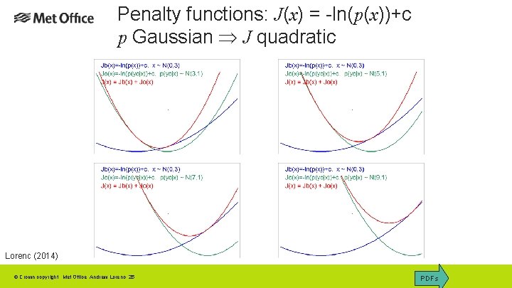
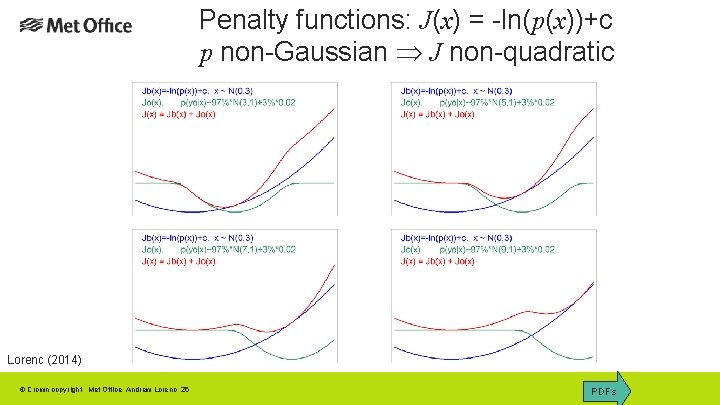
Variational Penalty Functions Finding the most probable posterior value involves maximising a product [of Gaussians] By taking –ln of the posterior PDF, we can instead minimise a sum This is often called the “Penalty Function” [of quadratics] J Additive constants can be ignored. Only implemented in Met Office system for scatterometer (Candy 2001). © Crown copyright Met Office Andrew Lorenc 24

Penalty functions: J(x) = -ln(p(x))+c p Gaussian J quadratic Lorenc (2014) © Crown copyright Met Office Andrew Lorenc 25 PDFs

Penalty functions: J(x) = -ln(p(x))+c p non-Gaussian J non-quadratic Lorenc (2014) © Crown copyright Met Office Andrew Lorenc 26 PDFs

Non-Gaussian DA. The need for QC of observations depends on the use being made of them. All observations can be plotted for human analysis – an experienced forecaster will allow for errors while drawing up weather chart. In contrast, “Objective” verification statistics are very sensitive to QC of verifying observations. Gaussian-based (least-squares) analysis methods have fairly clear requirements to reject observations which do not fit the Gaussian hypothesis. Non-Gaussian methods can allow directly for error properties, making a separate QC step unnecessary. © Crown copyright Met Office Andrew Lorenc 27

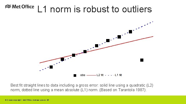
L 1 norm is robust to outliers Best fit straight lines to data including a gross error: solid line using a quadratic (L 2) norm, dotted line using a mean absolute (L 1) norm. (Based on Tarantola 1987). © Crown copyright Met Office Andrew Lorenc 28

Coping with multiply minima – finding best combination of inter-related decisions. Do a preliminary “pass” [with larger scale] before performing QC. Start with inflated observational errors, decreasing to correct values during the iteration (Dharssi et al. 1992) Only switch on variational QC after N (~20) iterations. Rely mainly on QC v background forecast (which is assumed to have Gaussian errors). Design iterative “buddy check” algorithm to start with easiest decisions. Change to robust DA algorithm (e. g. Huber norm). © Crown copyright Met Office Andrew Lorenc 29

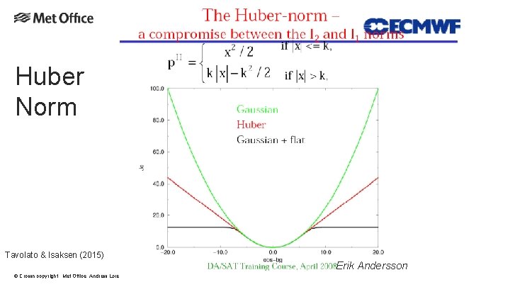
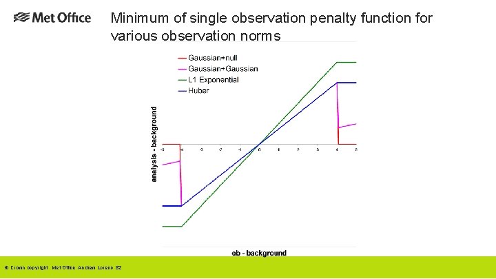
Models for Observation Error PDFs Gaussian + “null” prior. Simple. Assumes that erroneous observations do not add to prior knowledge. Used in most of my QC work. Problems normalising – does not integrate to 1. Gives multiple minima. Gaussian + wider Gaussian. Similar in practice to above. Normalised. Erroneous obs make small change to prior. Gives multiple minima. Back to back exponentials. Implied by use of L 1 norm (Tarantola 1987). Finds median – “pull” of all observations is equal. Not differentiable at origin, so difficult to minimise. Robust. Huber Norm. Huber (1973), Guitton and Symes (2003). Used at ECMWF. L 2 for small deviations, L 1 for large. Finds consensus average - “pull” of observations limited, rather than increasing indefinitely with misfit. Robust. © Crown copyright Met Office Andrew Lorenc 30

Huber Norm Tavolato & Isaksen (2015) © Crown copyright Met Office Andrew Lorenc 31 Erik Andersson

Minimum of single observation penalty function for various observation norms © Crown copyright Met Office Andrew Lorenc 32

Assessing the Value of Observations © Crown copyright Met Office Andrew Lorenc 33

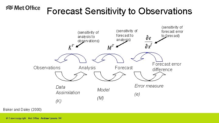
Forecast Sensitivity to Observations (sensitivity of analysis to observations) Observations Analysis Data Assimilation (K) Baker and Daley (2000) © Crown copyright Met Office Andrew Lorenc 34 (sensitivity of forecast to analysis) Forecast error difference Forecast Model (M) (sensitivity of forecast error to forecast) Error measure (e)

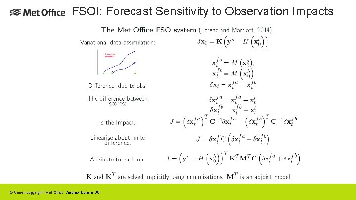
FSOI: Forecast Sensitivity to Observation Impacts © Crown copyright Met Office Andrew Lorenc 35

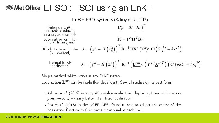
EFSOI: FSOI using an En. KF © Crown copyright Met Office Andrew Lorenc 36

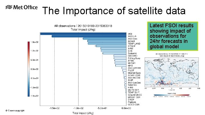
The Importance of satellite data Latest FSOI results showing impact of observations for 24 hr forecasts in global model © Crown copyright Met Office

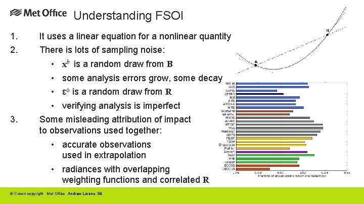
Understanding FSOI 1. 2. 3. It uses a linear equation for a nonlinear quantity There is lots of sampling noise: • xb is a random draw from B • some analysis errors grow, some decay • εo is a random draw from R • verifying analysis is imperfect Some misleading attribution of impact to observations used together: • accurate observations used in extrapolation • radiances with overlapping weighting functions and correlated R © Crown copyright Met Office Andrew Lorenc 38

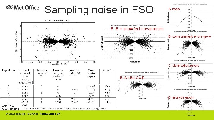
Sampling noise in FSOI A: none F: E + imperfect covariances B: some analysis errors grow C: observation errors E: A + B + C + D D: analysis errors Lorenc & Marriott 2014 © Crown copyright Met Office Andrew Lorenc 39

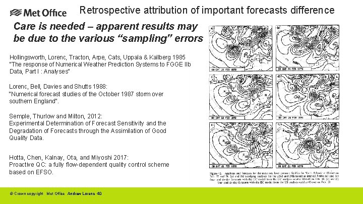
Retrospective attribution of important forecasts difference Care is needed – apparent results may be due to the various “sampling” errors Hollingsworth, Lorenc, Tracton, Arpe, Cats, Uppala & Kallberg 1985 "The response of Numerical Weather Prediction Systems to FGGE IIb Data, Part I : Analyses" Lorenc, Bell, Davies and Shutts 1988: "Numerical forecast studies of the October 1987 storm over southern England". Semple, Thurlow and Milton, 2012: Experimental Determination of Forecast Sensitivity and the Degradation of Forecasts through the Assimilation of Good Quality Data. Hotta, Chen, Kalnay, Ota, and Miyoshi 2017: Proactive QC: a fully flow-dependent quality control scheme based on EFSO. © Crown copyright Met Office Andrew Lorenc 40

Other methods for assessing observation impact OSE: Observing System Experiments. “What is the impact of omitted/adding OS on current NWP system? ” Measures impact of one OS on many scores. Expensive in computing. Usual by-product of trials of a new OS. OSSE: Observing System Simulation Experiments. Often used to answer “What would the impact be of a new OS on NWP skill in ~20 years time? ” Expensive in labour and computing. Needs expert interpretation/validation. DA Ensemble Spread (Tan et al. 2007): Uses real observations + simulated new system. Assesses impact via the reduction in analysis ensemble spread. Om. F statistics (Todling 2013): Avoids problems of FSOI, but only estimates potential impact, rather than actual impact. Compares innovation variances for different forecast lengths, and assumes that “Decrease in Om. F=<d 2> for an OS, due to a better Forecast” “Assimilating this OS would give a better Forecast”. © Crown copyright Met Office Andrew Lorenc 41

Targeted of Observations © Crown copyright Met Office

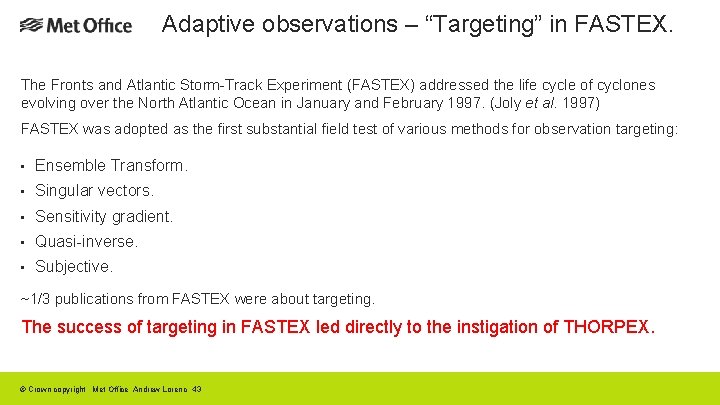
Adaptive observations – “Targeting” in FASTEX. The Fronts and Atlantic Storm-Track Experiment (FASTEX) addressed the life cycle of cyclones evolving over the North Atlantic Ocean in January and February 1997. (Joly et al. 1997) FASTEX was adopted as the first substantial field test of various methods for observation targeting: • Ensemble Transform. • Singular vectors. • Sensitivity gradient. • Quasi-inverse. • Subjective. ~1/3 publications from FASTEX were about targeting. The success of targeting in FASTEX led directly to the instigation of THORPEX. © Crown copyright Met Office Andrew Lorenc 43

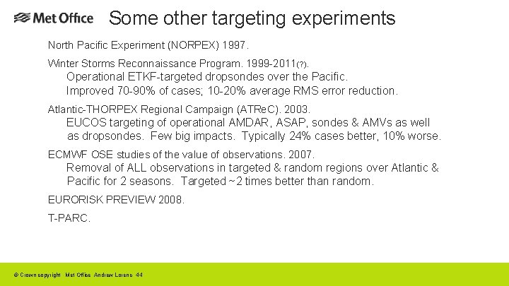
Some other targeting experiments North Pacific Experiment (NORPEX) 1997. Winter Storms Reconnaissance Program. 1999 -2011(? ). Operational ETKF-targeted dropsondes over the Pacific. Improved 70 -90% of cases; 10 -20% average RMS error reduction. Atlantic-THORPEX Regional Campaign (ATRe. C). 2003. EUCOS targeting of operational AMDAR, ASAP, sondes & AMVs as well as dropsondes. Few big impacts. Typically 24% cases better, 10% worse. ECMWF OSE studies of the value of observations. 2007. Removal of ALL observations in targeted & random regions over Atlantic & Pacific for 2 seasons. Targeted ~2 times better than random. EURORISK PREVIEW 2008. T-PARC. © Crown copyright Met Office Andrew Lorenc 44

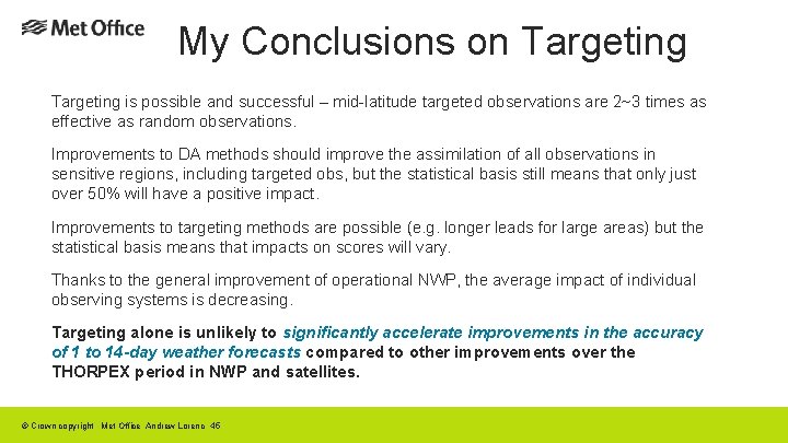
My Conclusions on Targeting is possible and successful – mid-latitude targeted observations are 2~3 times as effective as random observations. Improvements to DA methods should improve the assimilation of all observations in sensitive regions, including targeted obs, but the statistical basis still means that only just over 50% will have a positive impact. Improvements to targeting methods are possible (e. g. longer leads for large areas) but the statistical basis means that impacts on scores will vary. Thanks to the general improvement of operational NWP, the average impact of individual observing systems is decreasing. Targeting alone is unlikely to significantly accelerate improvements in the accuracy of 1 to 14 -day weather forecasts compared to other improvements over the THORPEX period in NWP and satellites. © Crown copyright Met Office Andrew Lorenc 45

Observing System Experiments © Crown copyright Met Office

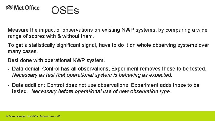
OSEs Measure the impact of observations on existing NWP systems, by comparing a wide range of scores with & without them. To get a statistically significant signal, have to do it on whole observing systems over many cases. Best done with operational NWP system. • Data denial: Control has all observations, Experiment removes those to be tested. Necessary as test that operational system is behaving as expected. • Data addition: Control does not use observations; Experiment adds those to be tested. Necessary before operational use of new observation type. © Crown copyright Met Office Andrew Lorenc 47

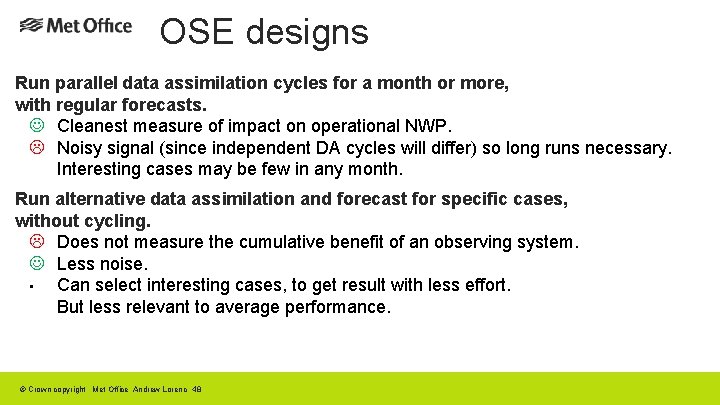
OSE designs Run parallel data assimilation cycles for a month or more, with regular forecasts. J Cleanest measure of impact on operational NWP. L Noisy signal (since independent DA cycles will differ) so long runs necessary. Interesting cases may be few in any month. Run alternative data assimilation and forecast for specific cases, without cycling. L Does not measure the cumulative benefit of an observing system. J Less noise. • Can select interesting cases, to get result with less effort. But less relevant to average performance. © Crown copyright Met Office Andrew Lorenc 48

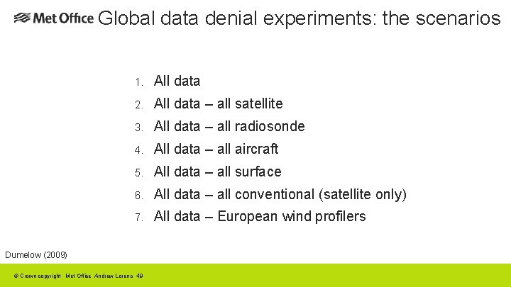
Global data denial experiments: the scenarios 1. All data 2. All data – all satellite 3. All data – all radiosonde 4. All data – all aircraft 5. All data – all surface 6. All data – all conventional (satellite only) 7. All data – European wind profilers Dumelow (2009) © Crown copyright Met Office Andrew Lorenc 49

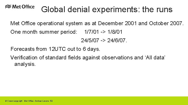
Global denial experiments: the runs Met Office operational system as at December 2001 and October 2007. One month summer period: 1/7/01 -> 1/8/01 24/5/07 -> 24/6/07. Forecasts from 12 UTC out to 6 days. Verification of standard fields against observations and ‘All data’ analysis. © Crown copyright Met Office Andrew Lorenc 50

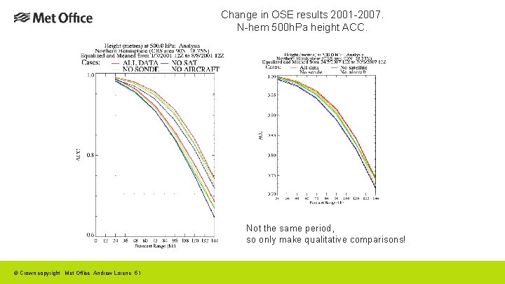
Change in OSE results 2001 -2007. N-hem 500 h. Pa height ACC. Not the same period, so only make qualitative comparisons! © Crown copyright Met Office Andrew Lorenc 51

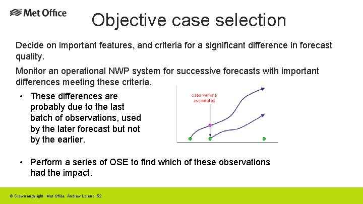
Objective case selection Decide on important features, and criteria for a significant difference in forecast quality. Monitor an operational NWP system for successive forecasts with important differences meeting these criteria. • These differences are probably due to the last batch of observations, used by the later forecast but not by the earlier. • Perform a series of OSE to find which of these observations had the impact. © Crown copyright Met Office Andrew Lorenc 52

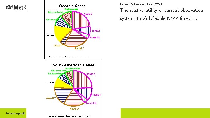
Graham Anderson and Bader (2000) The relative utility of current observation systems to global-scale NWP forecasts © Crown copyright Met Office Andrew Lorenc 53

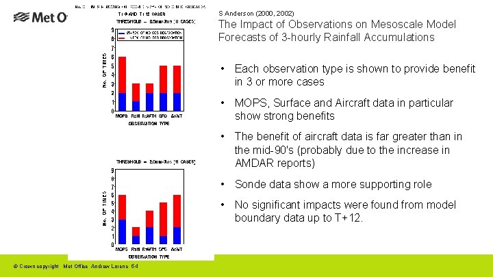
S Anderson (2000, 2002) The Impact of Observations on Mesoscale Model Forecasts of 3 -hourly Rainfall Accumulations • Each observation type is shown to provide benefit in 3 or more cases • MOPS, Surface and Aircraft data in particular show strong benefits • The benefit of aircraft data is far greater than in the mid-90's (probably due to the increase in AMDAR reports) • Sonde data show a more supporting role • No significant impacts were found from model boundary data up to T+12. © Crown copyright Met Office Andrew Lorenc 54

Observing System Simulation Experiments OSSEs © Crown copyright Met Office

OSSEs Allow us to estimate the impact of observing systems which do not yet exist. 1. Simple idealised experiments. What might be the impact of next generation satellite data on next generation NWP systems? 2. Full calibrated OSSEs. What is the impact of next generation satellite data on current NWP systems? © Crown copyright Met Office Andrew Lorenc 56

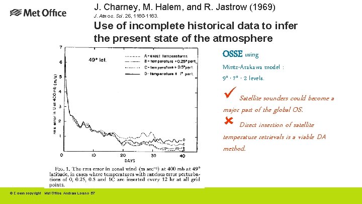
J. Charney, M. Halem, and R. Jastrow (1969) J. Atmos. Sci. 26, 1160 -1163. Use of incomplete historical data to infer the present state of the atmosphere OSSE using Mintz-Arakawa model : 9° 7° 2 levels. x x ü Satellite sounders could become a major part of the global OS. Direct insertion of satellite temperature retrievals is a viable DA method. û © Crown copyright Met Office Andrew Lorenc 57

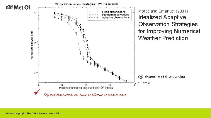
Morss and Emanuel (2001) Idealized Adaptive Observation Strategies for Improving Numerical Weather Prediction QG channel model: 250 km 5 levels x x ü Targeted observations are twice as effective as random ones. © Crown copyright Met Office Andrew Lorenc 58

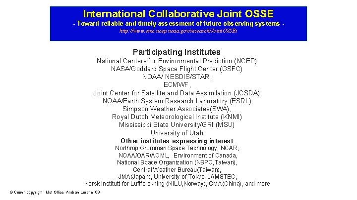
International Collaborative Joint OSSE - Toward reliable and timely assessment of future observing systems http: //www. emc. ncep. noaa. gov/research/Joint. OSSEs Participating Institutes National Centers for Environmental Prediction (NCEP) NASA/Goddard Space Flight Center (GSFC) NOAA/ NESDIS/STAR, ECMWF, Joint Center for Satellite and Data Assimilation (JCSDA) NOAA/Earth System Research Laboratory (ESRL) Simpson Weather Associates(SWA), Royal Dutch Meteorological Institute (KNMI) Mississippi State University/GRI (MSU) University of Utah Other institutes expressing interest Northrop Grumman Space Technology, NCAR, NOAA/OAR/AOML, Environment of Canada, National Space Organization (NSPO, Taiwan), Central Weather Bureau(Taiwan), JMA(Japan), University of Tokyo, JAMSTEC, Norsk Institutt for Luftforskning (NILU, Norway), CMA(China), and more © Crown copyright Met Office Andrew Lorenc 59

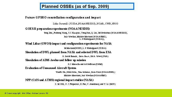
Planned OSSEs (as of Sep. 2009) Future GPSRO constellation configuration and impact Lidia Cucurull (JCSDA, NOAA/NESDIS), NCAR, CWB, NPSO GOES-R preparation experiments (NOAA/NESDIS) Tong Zhu, , Fuzhong Weng, T. J. Kleespies, Yong Han, Q. Liu, Sid Boukabara (NOAA/NESDIS), Jack Woollen, Michiko Masutani (NOAA/EMC), L. P Riishojgaard (JCSDA)), Wind Lidar (GWOS) impact and configuration experiments for NASA M. Masutani(NCEP), L. P Riishojgaard (JCSDA) Simulation of DWL planned from NASA and selected DWL from ESA G. David Emmitt, Steve Greco, Sid A. Wood, (SWA) Simulation of ADM-Aeolus and follow up mission G. J. Marseille and Ad Stoffelen (KNMI) Evaluation of Unmanned Aircraft System Yuanfu Xie, Nikki Prive, Tom Schlatter, Steve Koch (NOAA/ESRL) Michiko Matsutani, Jack Woollen (NOAA/EMC) NPP (Cr. IS and ATMS) regional impact studies (NASA) C. M. Hill, P. J. Fitzpatrick, X. Fan, V. Anantharaj, and Y. Li (MSU) © Crown copyright Met Office Andrew Lorenc 60

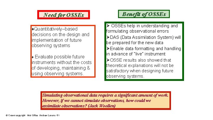
Need for OSSEs ♦Quantitatively–based decisions on the design and implementation of future observing systems ♦ Evaluate possible future instruments without the costs of developing, maintaining & using observing systems. Benefit of OSSEs Ø OSSEs help in understanding and formulating observational errors ØDAS (Data Assimilation System) will be prepared for the new data ØEnable data formatting and handling in advance of “live” instrument ØOSSE results also showed that theoretical explanations will not be satisfactory when designing future observing systems. Simulating observational data requires a significant amount of work. However, if we cannot simulate observations, how could we assimilate observations? (Jack Woollen) © Crown copyright Met Office Andrew Lorenc 61

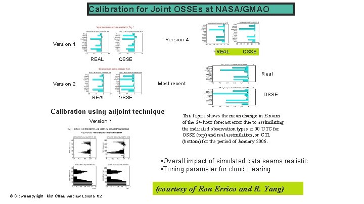
Calibration for Joint OSSEs at NASA/GMAO Version 4 Version 1 REAL OSSE Real Most recent Version 2 REAL OSSE Calibration using adjoint technique Version 1 This figure shows the mean change in E-norm of the 24 -hour forecast error due to assimilating the indicated observation types at 00 UTC for OSSE (top) and real assimilation, or CTL (bottom) for the period of January 2006. • Overall impact of simulated data seems realistic • Tuning parameter for cloud clearing (courtesy of Ron Errico and R. Yang) © Crown copyright Met Office Andrew Lorenc 62

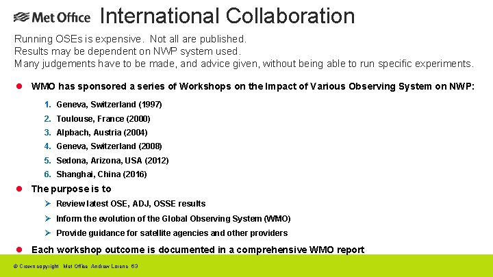
International Collaboration Running OSEs is expensive. Not all are published. Results may be dependent on NWP system used. Many judgements have to be made, and advice given, without being able to run specific experiments. l WMO has sponsored a series of Workshops on the Impact of Various Observing System on NWP: 1. Geneva, Switzerland (1997) 2. Toulouse, France (2000) 3. Alpbach, Austria (2004) 4. Geneva, Switzerland (2008) 5. Sedona, Arizona, USA (2012) 6. Shanghai, China (2016) l The purpose is to Ø Review latest OSE, ADJ, OSSE results Ø Inform the evolution of the Global Observing System (WMO) Ø Provide guidance for satellite agencies and other providers l Each workshop outcome is documented in a comprehensive WMO report © Crown copyright Met Office Andrew Lorenc 63

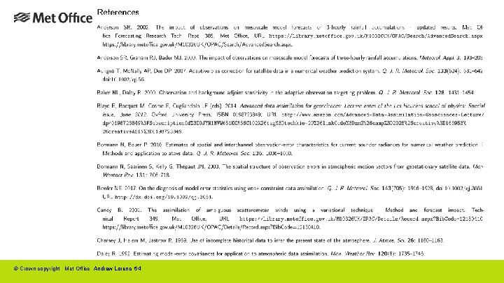
© Crown copyright Met Office Andrew Lorenc 64

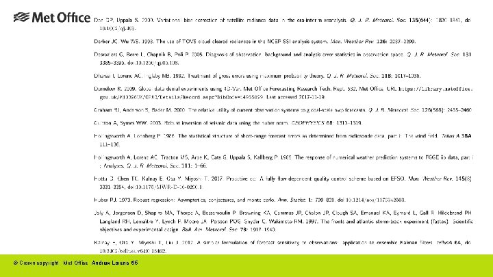
© Crown copyright Met Office Andrew Lorenc 65

© Crown copyright Met Office Andrew Lorenc 66

© Crown copyright Met Office Andrew Lorenc 67