Data Analytics CS 40003 Lecture 11 Sensitivity Analysis

Data Analytics (CS 40003) Lecture #11 Sensitivity Analysis Dr. Debasis Samanta Associate Professor Department of Computer Science & Engineering

Topics Covered in this Presentation � Introduction � Estimation Strategies � Accuracy Estimation � Error Estimation � Statistical Estimation � Performance Estimation � ROC Curve CS 40003: Data Analytics 2

Introduction � A classifier is used to predict an outcome of a test data � Such a prediction is useful in many applications � Business forecasting, cause-and-effect analysis, etc. � A number of classifiers have been evolved to support the activities. � Each has their own merits and demerits � There is a need to estimate the accuracy and performance of the classifier with respect to few controlling parameters in data sensitivity � As a task of sensitivity analysis, we have to focus on � Estimation strategy � Metrics for measuring accuracy � Metrics for measuring performance CS 40003: Data Analytics 3

Estimation Strategy CS 40003: Data Analytics 4

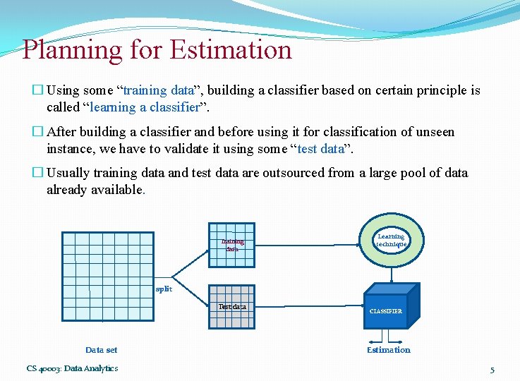
Planning for Estimation � Using some “training data”, building a classifier based on certain principle is called “learning a classifier”. � After building a classifier and before using it for classification of unseen instance, we have to validate it using some “test data”. � Usually training data and test data are outsourced from a large pool of data already available. Training data Learning technique split Test data Data set CS 40003: Data Analytics CLASSIFIER Estimation 5

Estimation Strategies � Accuracy and performance measurement should follow a strategy. As the topic is important, many strategies have been advocated so far. Most widely used strategies are � Holdout method � Random subsampling � Cross-validation � Bootstrap approach CS 40003: Data Analytics 6

Holdout Method � This is a basic concept of estimating a prediction. � Given a dataset, it is partitioned into two disjoint sets called training set and testing set. � Classifier is learned based on the training set and get evaluated with testing set. � Proportion of training and testing sets is at the discretion of analyst; typically 1: 1 or 2: 1, and there is a trade-off between these sizes of these two sets. � If the training set is too large, then model may be good enough, but estimation may be less reliable due to small testing set and vice-versa. CS 40003: Data Analytics 7

Random Subsampling � It is a variation of Holdout method to overcome the drawback of overpresenting a class in one set thus under-presenting it in the other set and vice-versa. � In this method, Holdout method is repeated k times, and in each time, two disjoint sets are chosen at random with a predefined sizes. � Overall estimation is taken as the average of estimations obtained from each iteration. CS 40003: Data Analytics 8

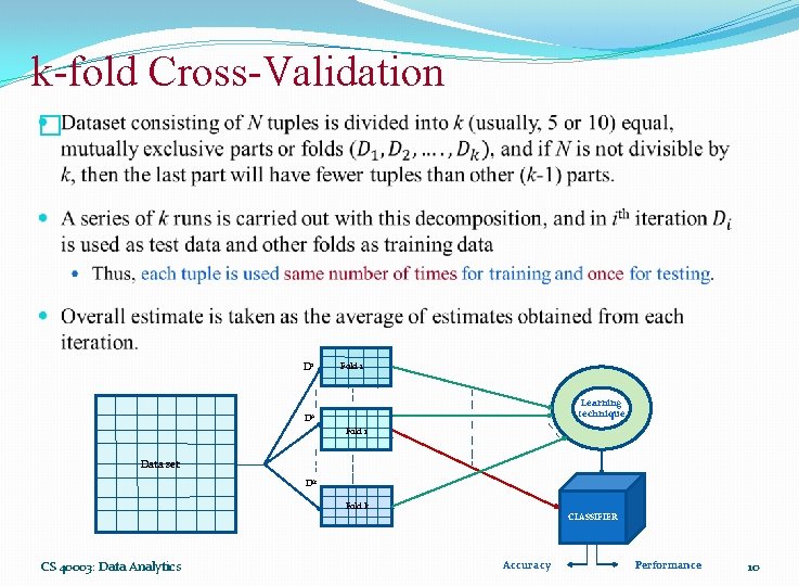
Cross-Validation � The main drawback of Random subsampling is, it does not have control over the number of times each tuple is used for training and testing. � Cross-validation is proposed to overcome this problem. � There are two variations in the cross-validation method. � k-fold cross-validation � N-fold cross-validation CS 40003: Data Analytics 9

k-fold Cross-Validation � D 1 Fold 1 Learning technique Di Fold i Data set Dk Fold k CLASSIFIER CS 40003: Data Analytics Accuracy Performance 10

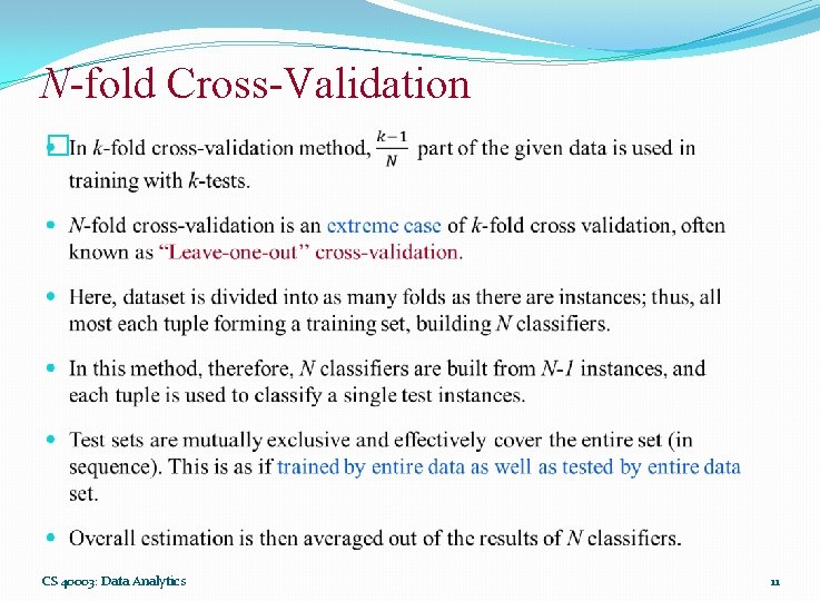
N-fold Cross-Validation � CS 40003: Data Analytics 11

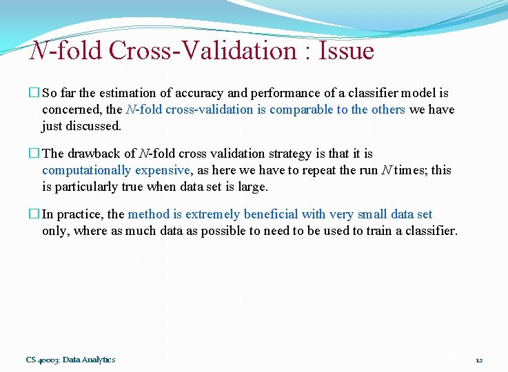
N-fold Cross-Validation : Issue � So far the estimation of accuracy and performance of a classifier model is concerned, the N-fold cross-validation is comparable to the others we have just discussed. � The drawback of N-fold cross validation strategy is that it is computationally expensive, as here we have to repeat the run N times; this is particularly true when data set is large. � In practice, the method is extremely beneficial with very small data set only, where as much data as possible to need to be used to train a classifier. CS 40003: Data Analytics 12

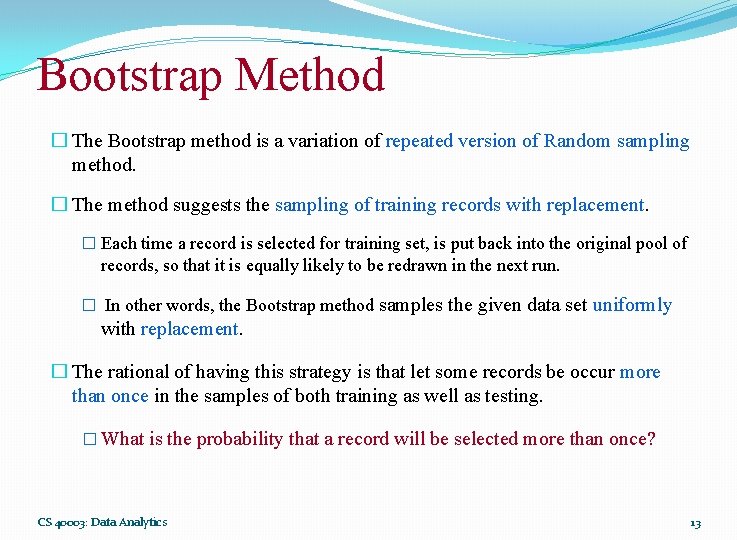
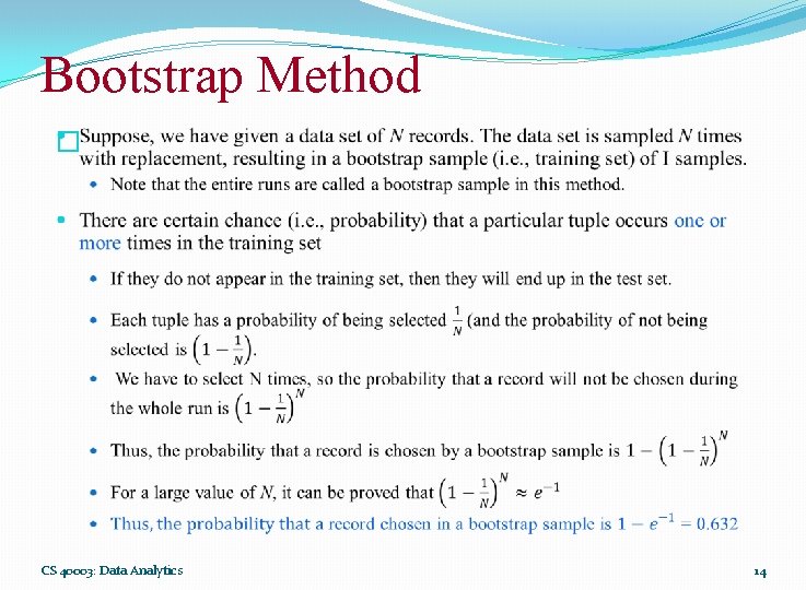
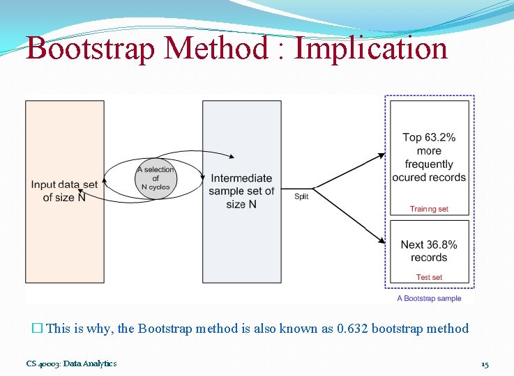
Bootstrap Method � The Bootstrap method is a variation of repeated version of Random sampling method. � The method suggests the sampling of training records with replacement. � Each time a record is selected for training set, is put back into the original pool of records, so that it is equally likely to be redrawn in the next run. � In other words, the Bootstrap method samples the given data set uniformly with replacement. � The rational of having this strategy is that let some records be occur more than once in the samples of both training as well as testing. � What is the probability that a record will be selected more than once? CS 40003: Data Analytics 13

Bootstrap Method � CS 40003: Data Analytics 14

Bootstrap Method : Implication � This is why, the Bootstrap method is also known as 0. 632 bootstrap method CS 40003: Data Analytics 15

Accuracy Estimation CS 40003: Data Analytics 16

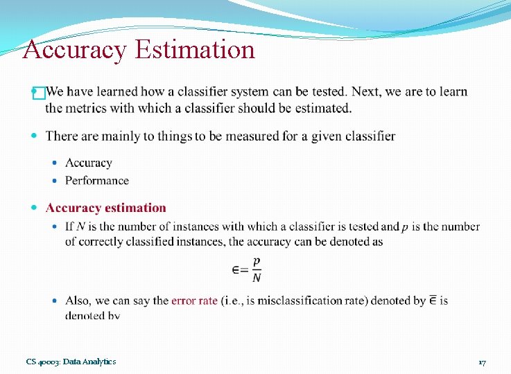
Accuracy Estimation � CS 40003: Data Analytics 17

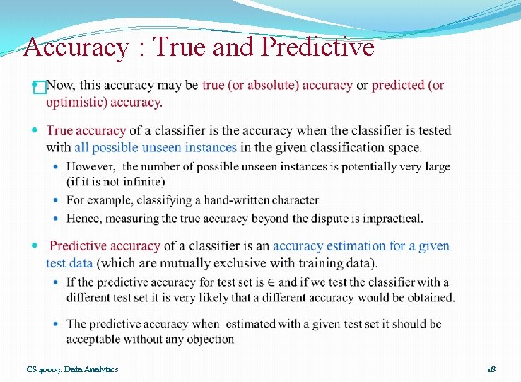
Accuracy : True and Predictive � CS 40003: Data Analytics 18

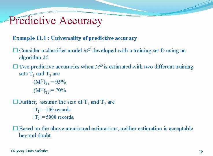
Predictive Accuracy Example 11. 1 : Universality of predictive accuracy � Consider a classifier model MD developed with a training set D using an algorithm M. � Two predictive accuracies when MD is estimated with two different training sets T 1 and T 2 are (MD)T 1 = 95% (MD)T 2 = 70% � Further, assume the size of T 1 and T 2 are |T 1| = 100 records |T 2| = 5000 records. � Based on the above mentioned estimations, neither estimation is acceptable beyond doubt. CS 40003: Data Analytics 19

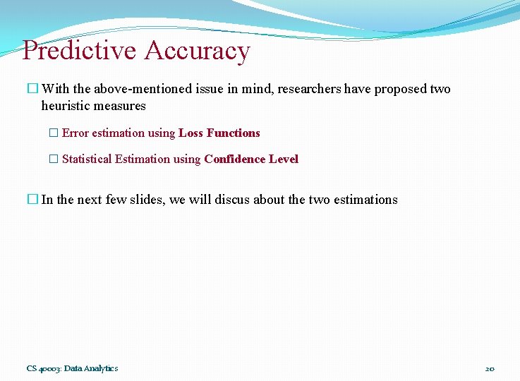
Predictive Accuracy � With the above-mentioned issue in mind, researchers have proposed two heuristic measures � Error estimation using Loss Functions � Statistical Estimation using Confidence Level � In the next few slides, we will discus about the two estimations CS 40003: Data Analytics 20

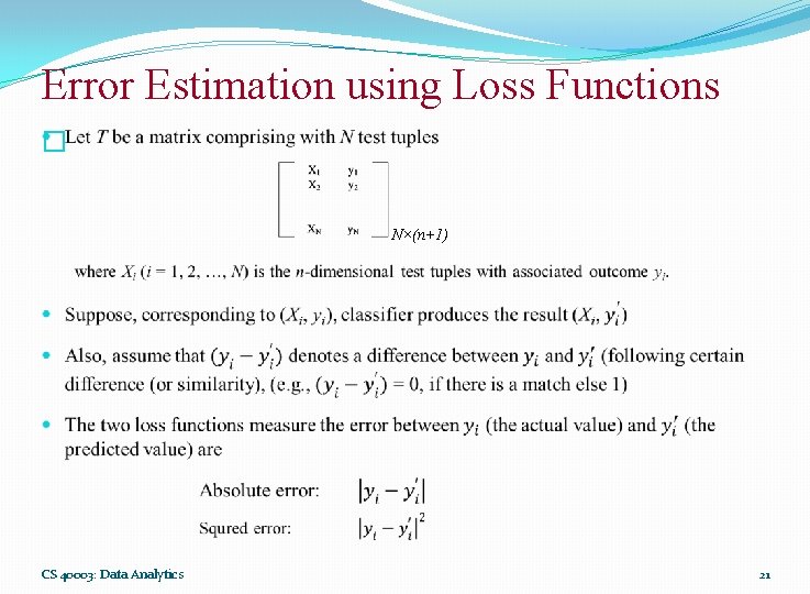
Error Estimation using Loss Functions � N×(n+1) CS 40003: Data Analytics 21

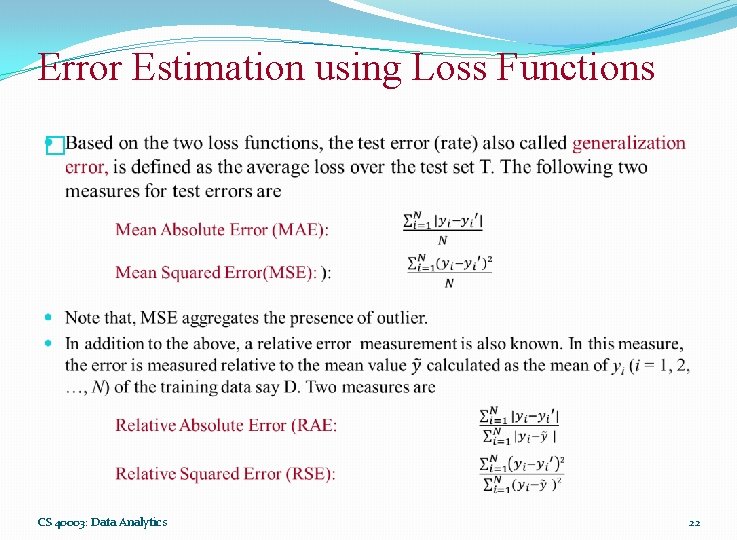
Error Estimation using Loss Functions � CS 40003: Data Analytics 22

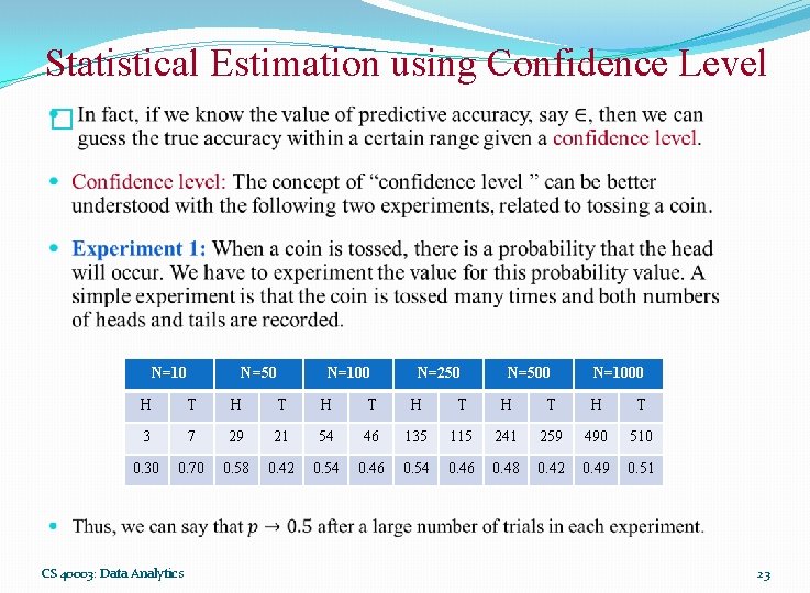
Statistical Estimation using Confidence Level � N=10 N=50 N=100 N=250 N=500 N=1000 H T H T H T 3 7 29 21 54 46 135 115 241 259 490 510 0. 30 0. 70 0. 58 0. 42 0. 54 0. 46 0. 48 0. 42 0. 49 0. 51 CS 40003: Data Analytics 23

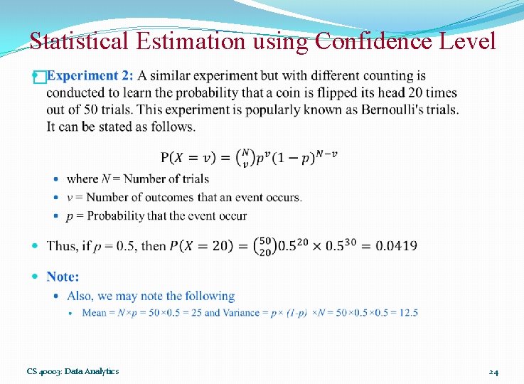
Statistical Estimation using Confidence Level � CS 40003: Data Analytics 24

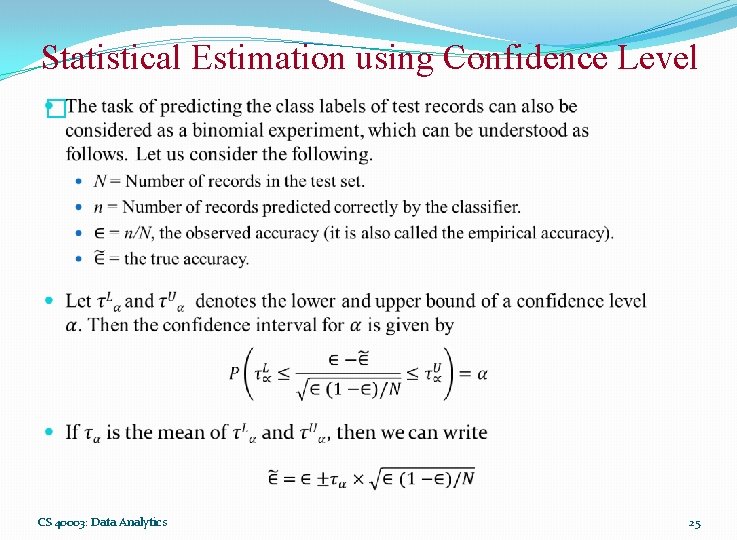
Statistical Estimation using Confidence Level � CS 40003: Data Analytics 25

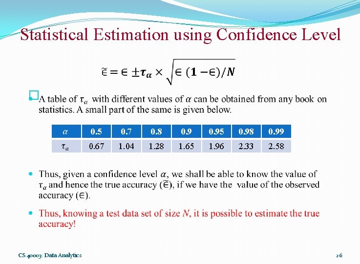
Statistical Estimation using Confidence Level � CS 40003: Data Analytics 0. 5 0. 7 0. 8 0. 95 0. 98 0. 99 0. 67 1. 04 1. 28 1. 65 1. 96 2. 33 2. 58 26

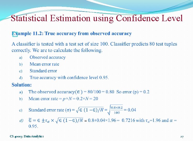
Statistical Estimation using Confidence Level � CS 40003: Data Analytics 27

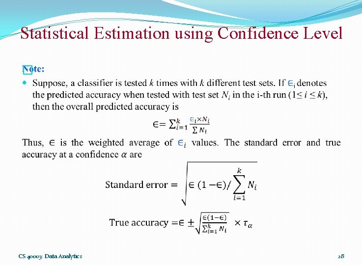
Statistical Estimation using Confidence Level � CS 40003: Data Analytics 28

Performance Estimation CS 40003: Data Analytics 29

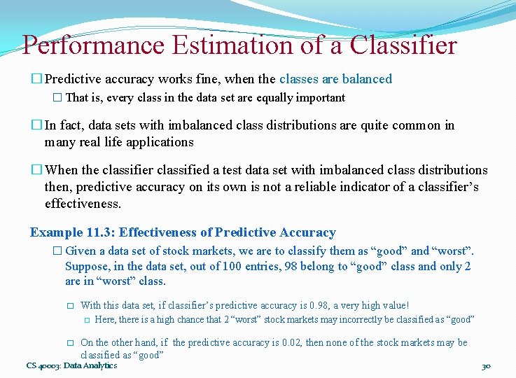
Performance Estimation of a Classifier � Predictive accuracy works fine, when the classes are balanced � That is, every class in the data set are equally important � In fact, data sets with imbalanced class distributions are quite common in many real life applications � When the classifier classified a test data set with imbalanced class distributions then, predictive accuracy on its own is not a reliable indicator of a classifier’s effectiveness. Example 11. 3: Effectiveness of Predictive Accuracy � Given a data set of stock markets, we are to classify them as “good” and “worst”. Suppose, in the data set, out of 100 entries, 98 belong to “good” class and only 2 are in “worst” class. � With this data set, if classifier’s predictive accuracy is 0. 98, a very high value! � � Here, there is a high chance that 2 “worst” stock markets may incorrectly be classified as “good” On the other hand, if the predictive accuracy is 0. 02, then none of the stock markets may be classified as “good” CS 40003: Data Analytics 30

Performance Estimation of a Classifier � Thus, when the classifier classified a test data set with imbalanced class distributions, then predictive accuracy on its own is not a reliable indicator of a classifier’s effectiveness. � This necessitates an alternative metrics to judge the classifier. � Before exploring them, we introduce the concept of Confusion matrix. CS 40003: Data Analytics 31

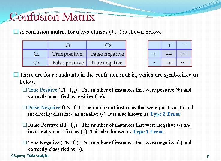
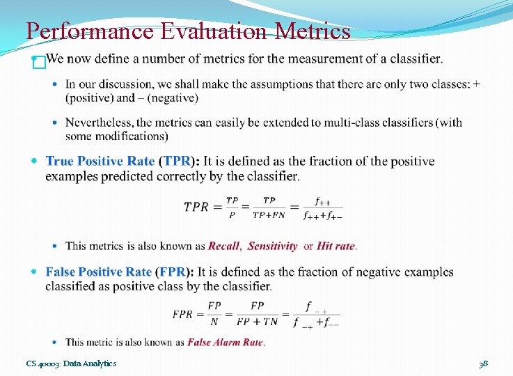
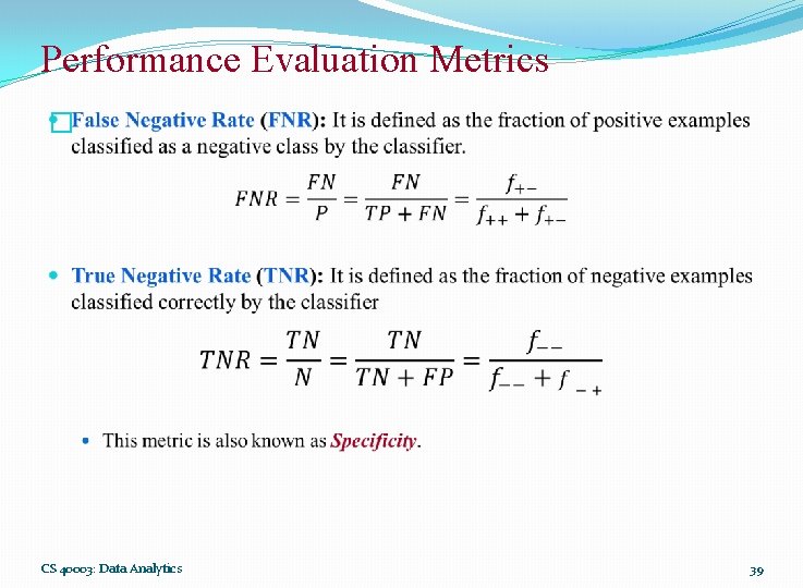
Confusion Matrix � A confusion matrix for a two classes (+, -) is shown below. � There are four quadrants in the confusion matrix, which are symbolized as below. � True Positive (TP: f++) : The number of instances that were positive (+) and correctly classified as positive (+v). � False Negative (FN: f+-): The number of instances that were positive (+) and incorrectly classified as negative (-). It is also known as Type 2 Error. � False Positive (FP: f-+): The number of instances that were negative (-) and incorrectly classified as (+). This also known as Type 1 Error. � True Negative (TN: f--): The number of instances that were negative (-) and correctly classified as (-). CS 40003: Data Analytics 32

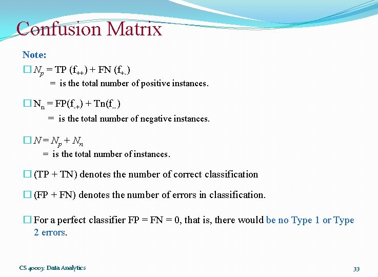
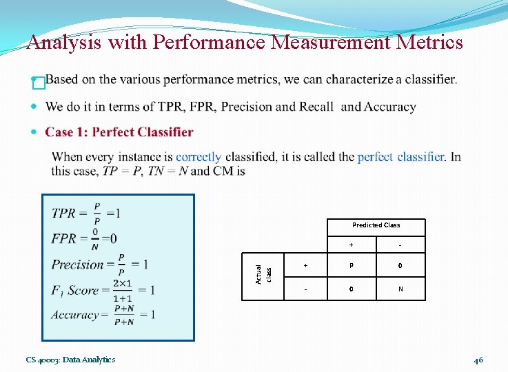
Confusion Matrix Note: � Np = TP (f++) + FN (f+-) = is the total number of positive instances. � Nn = FP(f-+) + Tn(f--) = is the total number of negative instances. � N = Np + Nn = is the total number of instances. � (TP + TN) denotes the number of correct classification � (FP + FN) denotes the number of errors in classification. � For a perfect classifier FP = FN = 0, that is, there would be no Type 1 or Type 2 errors. CS 40003: Data Analytics 33

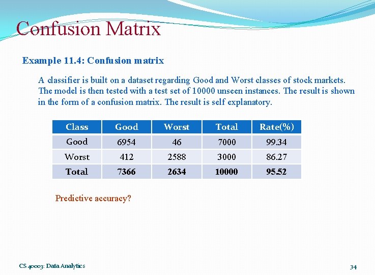
Confusion Matrix Example 11. 4: Confusion matrix A classifier is built on a dataset regarding Good and Worst classes of stock markets. The model is then tested with a test set of 10000 unseen instances. The result is shown in the form of a confusion matrix. The result is self explanatory. Class Good Worst Total Rate(%) Good 6954 46 7000 99. 34 Worst 412 2588 3000 86. 27 Total 7366 2634 10000 95. 52 Predictive accuracy? CS 40003: Data Analytics 34

Confusion Matrix for Multiclass Classifier � Having m classes, confusion matrix is a table of size m×m , where, element at (i, j) indicates the number of instances of class i but classified as class j. � To have good accuracy for a classifier, ideally most diagonal entries should have large values with the rest of entries being close to zero. � Confusion matrix may have additional rows or columns to provide total or recognition rates per class. CS 40003: Data Analytics 35

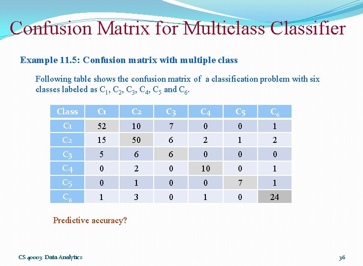
Confusion Matrix for Multiclass Classifier Example 11. 5: Confusion matrix with multiple class Following table shows the confusion matrix of a classification problem with six classes labeled as C 1, C 2, C 3, C 4, C 5 and C 6. Class C 1 C 2 C 3 C 4 C 5 C 6 C 1 52 10 7 0 0 1 C 2 15 50 6 2 1 2 C 3 5 6 6 0 0 0 C 4 0 2 0 10 0 1 C 5 0 1 0 0 7 1 C 6 1 3 0 1 0 24 Predictive accuracy? CS 40003: Data Analytics 36

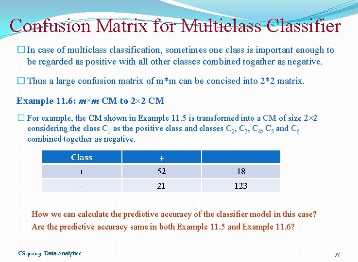
Confusion Matrix for Multiclass Classifier � In case of multiclassification, sometimes one class is important enough to be regarded as positive with all other classes combined togather as negative. � Thus a large confusion matrix of m*m can be concised into 2*2 matrix. Example 11. 6: m×m CM to 2× 2 CM � For example, the CM shown in Example 11. 5 is transformed into a CM of size 2× 2 considering the class C 1 as the positive class and classes C 2, C 3, C 4, C 5 and C 6 combined together as negative. Class + - + 52 18 - 21 123 How we can calculate the predictive accuracy of the classifier model in this case? Are the predictive accuracy same in both Example 11. 5 and Example 11. 6? CS 40003: Data Analytics 37

Performance Evaluation Metrics � CS 40003: Data Analytics 38

Performance Evaluation Metrics � CS 40003: Data Analytics 39

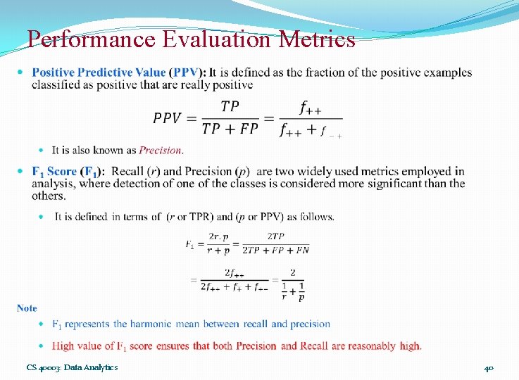
Performance Evaluation Metrics CS 40003: Data Analytics 40

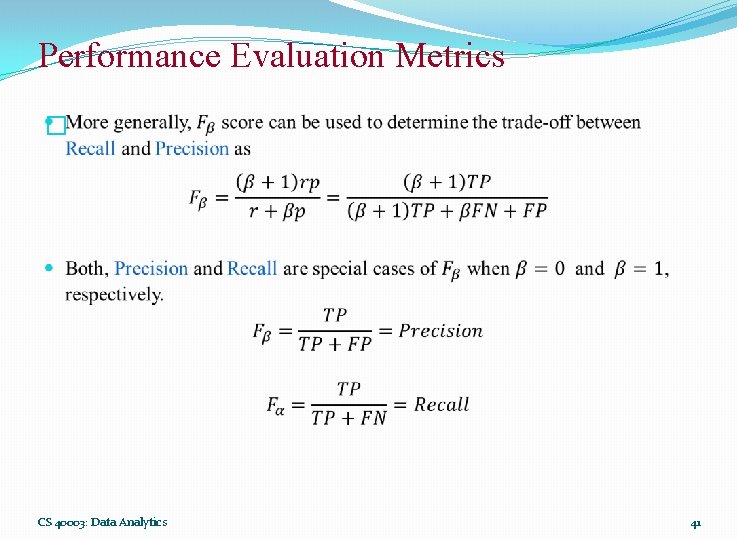
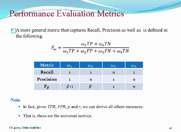
Performance Evaluation Metrics � CS 40003: Data Analytics 41

Performance Evaluation Metrics � Metric Recall 1 1 0 1 Precision 1 0 1 0 CS 40003: Data Analytics 42

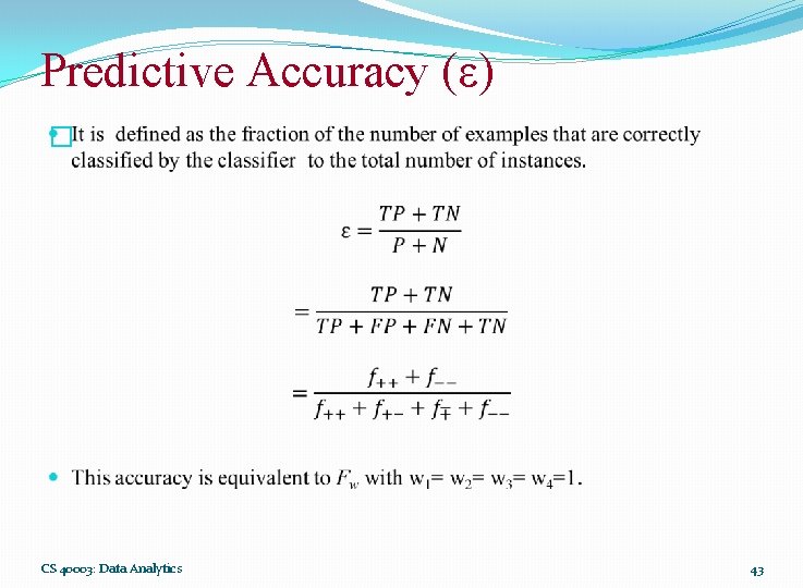
Predictive Accuracy (ε) � CS 40003: Data Analytics 43

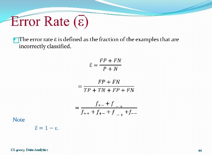
� CS 40003: Data Analytics 44

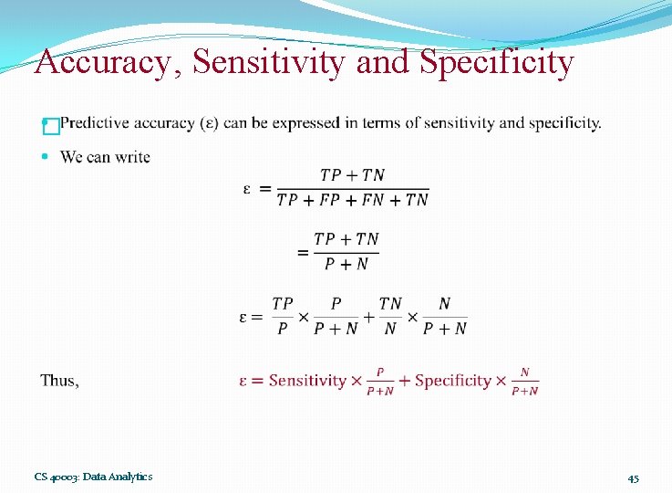
Accuracy, Sensitivity and Specificity � CS 40003: Data Analytics 45

Analysis with Performance Measurement Metrics � Actual class CS 40003: Data Analytics Predicted Class + - + P 0 - 0 N 46

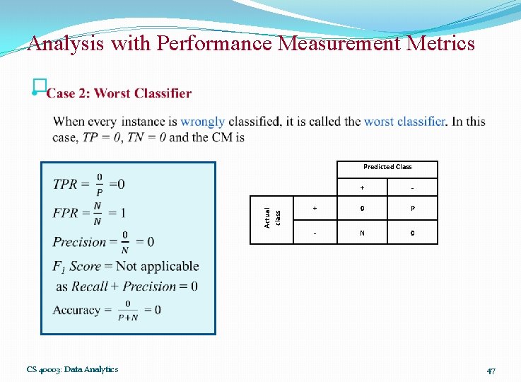
Analysis with Performance Measurement Metrics � Actual class CS 40003: Data Analytics Predicted Class + - + 0 P - N 0 47

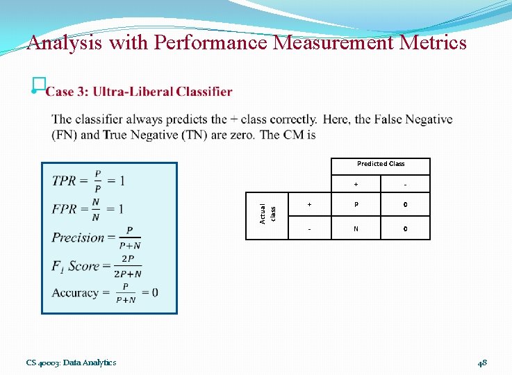
Analysis with Performance Measurement Metrics � Actual class CS 40003: Data Analytics Predicted Class + - + P 0 - N 0 48

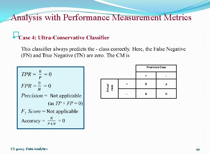
Analysis with Performance Measurement Metrics � Actual class CS 40003: Data Analytics Predicted Class + - + 0 p - 0 N 49

Predictive Accuracy versus TPR and FPR � One strength of characterizing a classifier by its TPR and FPR is that they do not depend on the relative size of P and N. � The same is also applicable for FNR and TNR and others measures from CM. � In contrast, the Predictive Accuracy, Precision, Error Rate, F 1 Score, etc. are affected by the relative size of P and N. � FPR, TPR, FNR and TNR are calculated from the different rows of the CM. � On the other hand Predictive Accuracy, etc. are derived from the values in both rows. � This suggests that FPR, TPR, FNR and TNR are more effective than Predictive Accuracy, etc. CS 40003: Data Analytics 50

ROC Curves CS 40003: Data Analytics 51

ROC Curves � ROC is an abbreviation of Receiver Operating Characteristic come from the signal detection theory, developed during World War 2 for analysis of radar images. � In the context of classifier, ROC plot is a useful tool to study the behaviour of a classifier or comparing two or more classifiers. � A ROC plot is a two-dimensional graph, where, X-axis represents FP rate (FPR) and Y-axis represents TP rate (TPR). � Since, the values of FPR and TPR varies from 0 to 1 both inclusive, the two axes thus from 0 to 1 only. � Each point (x, y) on the plot indicating that the FPR has value x and the TPR value y. CS 40003: Data Analytics 52

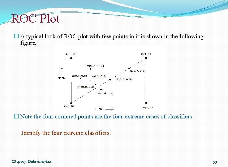
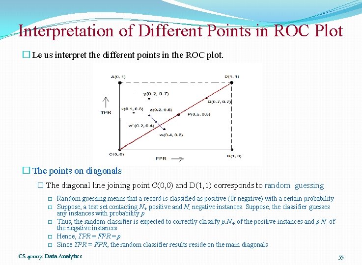
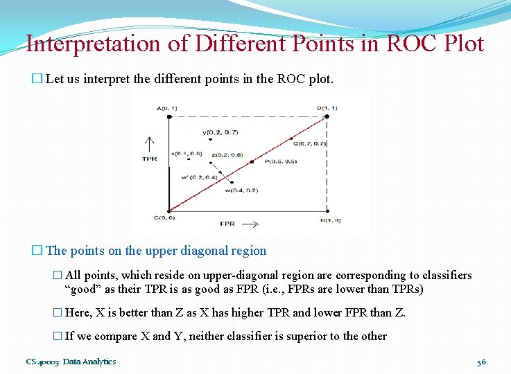
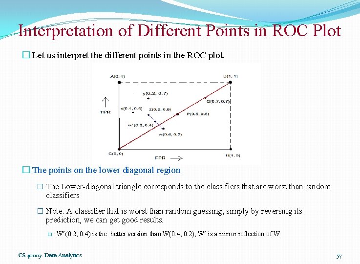
ROC Plot � A typical look of ROC plot with few points in it is shown in the following figure. � Note the four cornered points are the four extreme cases of classifiers Identify the four extreme classifiers. CS 40003: Data Analytics 53

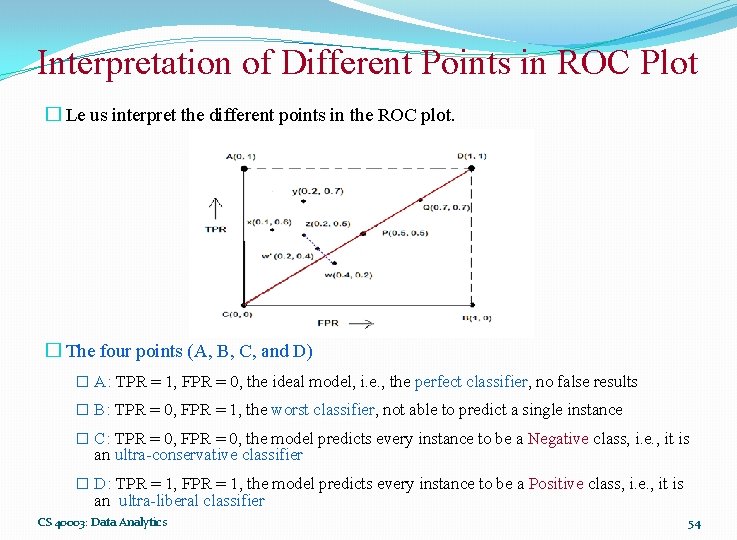
Interpretation of Different Points in ROC Plot � Le us interpret the different points in the ROC plot. � The four points (A, B, C, and D) � A: TPR = 1, FPR = 0, the ideal model, i. e. , the perfect classifier, no false results � B: TPR = 0, FPR = 1, the worst classifier, not able to predict a single instance � C: TPR = 0, FPR = 0, the model predicts every instance to be a Negative class, i. e. , it is an ultra-conservative classifier � D: TPR = 1, FPR = 1, the model predicts every instance to be a Positive class, i. e. , it is an ultra-liberal classifier CS 40003: Data Analytics 54

Interpretation of Different Points in ROC Plot � Le us interpret the different points in the ROC plot. � The points on diagonals � The diagonal line joining point C(0, 0) and D(1, 1) corresponds to random guessing � � � Random guessing means that a record is classified as positive (0 r negative) with a certain probability Suppose, a test set contacting N+ positive and N- negative instances. Suppose, the classifier guesses any instances with probability p Thus, the random classifier is expected to correctly classify p. N+ of the positive instances and p. N- of the negative instances Hence, TPR = FPR = p Since TPR = FPR, the random classifier results reside on the main diagonals CS 40003: Data Analytics 55

Interpretation of Different Points in ROC Plot � Let us interpret the different points in the ROC plot. � The points on the upper diagonal region � All points, which reside on upper-diagonal region are corresponding to classifiers “good” as their TPR is as good as FPR (i. e. , FPRs are lower than TPRs) � Here, X is better than Z as X has higher TPR and lower FPR than Z. � If we compare X and Y, neither classifier is superior to the other CS 40003: Data Analytics 56

Interpretation of Different Points in ROC Plot � Let us interpret the different points in the ROC plot. � The points on the lower diagonal region � The Lower-diagonal triangle corresponds to the classifiers that are worst than random classifiers � Note: A classifier that is worst than random guessing, simply by reversing its prediction, we can get good results. � W’(0. 2, 0. 4) is the better version than W(0. 4, 0. 2), W’ is a mirror reflection of W CS 40003: Data Analytics 57

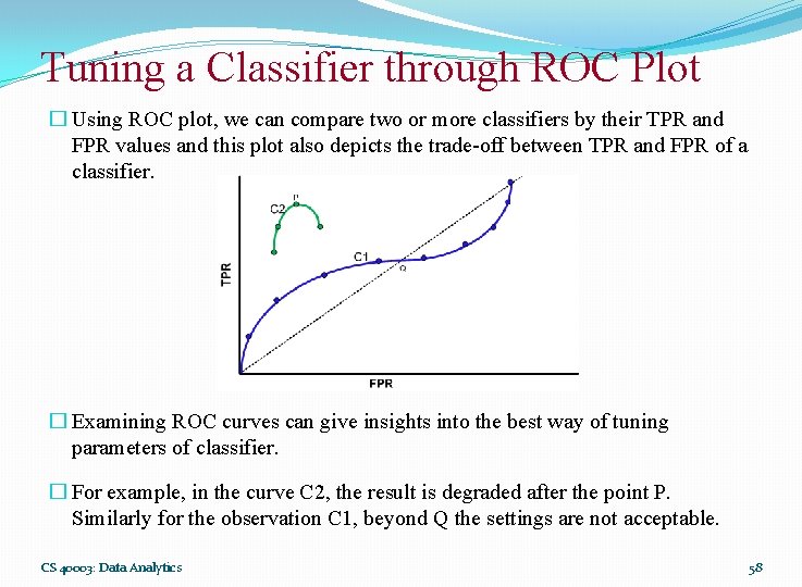
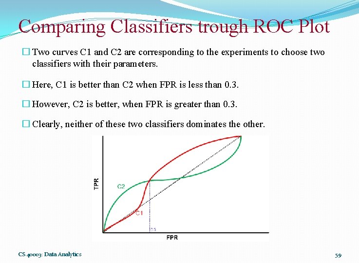
Tuning a Classifier through ROC Plot � Using ROC plot, we can compare two or more classifiers by their TPR and FPR values and this plot also depicts the trade-off between TPR and FPR of a classifier. � Examining ROC curves can give insights into the best way of tuning parameters of classifier. � For example, in the curve C 2, the result is degraded after the point P. Similarly for the observation C 1, beyond Q the settings are not acceptable. CS 40003: Data Analytics 58

Comparing Classifiers trough ROC Plot � Two curves C 1 and C 2 are corresponding to the experiments to choose two classifiers with their parameters. � Here, C 1 is better than C 2 when FPR is less than 0. 3. � However, C 2 is better, when FPR is greater than 0. 3. � Clearly, neither of these two classifiers dominates the other. CS 40003: Data Analytics 59

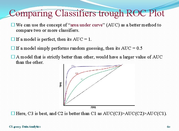
Comparing Classifiers trough ROC Plot � We can use the concept of “area under curve” (AUC) as a better method to compare two or more classifiers. � If a model is perfect, then its AUC = 1. � If a model simply performs random guessing, then its AUC = 0. 5 � A model that is strictly better than other, would have a larger value of AUC than the other. � Here, C 3 is best, and C 2 is better than C 1 as AUC(C 3)>AUC(C 2)>AUC(C 1). CS 40003: Data Analytics 60

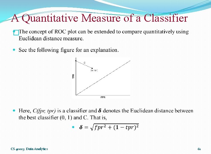
A Quantitative Measure of a Classifier � CS 40003: Data Analytics 61

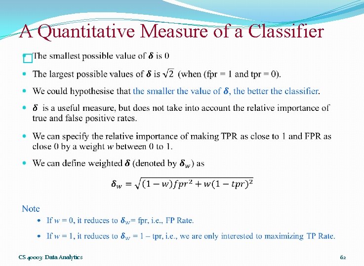
A Quantitative Measure of a Classifier � CS 40003: Data Analytics 62

Reference � The detail material related to this lecture can be found in Data Mining: Concepts and Techniques, (3 rd Edn. ), Jiawei Han, Micheline Kamber, Morgan Kaufmann, 2015. Introduction to Data Mining, Pang-Ning Tan, Michael Steinbach, and Vipin Kumar, Addison-Wesley, 2014 CS 40003: Data Analytics 63

Any question? You may post your question(s) at the “Discussion Forum” maintained in the course Web page! CS 40003: Data Analytics 64