Data analysis using R Jasminka Doba Faculty of

Data analysis using R Jasminka Dobša Faculty of Organization and Informatics University of Zagreb Workshop on Data Analysis 2018 1

Outline • Introduction to R • Descriptive statistics and graphical representation of data • Random variables and probability distributuions § Binomial distribution § Normal distribution • Testing the normality of distribution • Statistical testing • Testing of means for two populations § T-test and similar nonparametric tests • Testing of dependence of two qualitative variables § Chi-square test 2 Workshop on Data Analysis 2018

What is R? • R is an integrated package of program contents for data analysis • Enables: § § Handling data and storing them Graphic representation, visualization of data Operation over the sequences and matrices Data analysis using statistical and data mining methods • Contains a simple and efficient programming language (S) • It can be considered as implementing S programming language 3 Workshop on Data Analysis 2018

Instalation and links • We will use § R, RCommander (graphical interface for R-use) § RStudio: environment for R-use • Instalation: § 1 st step: R project (https: //www. r-project. org/) § 2 nd step: RStudio (https: //www. rstudio. com/products/rstudio/download/ • Tutorials for R i RStudio (47 videos) by Mike Marin https: //www. youtube. com/watch? v=c. X 532 N_XLIs&list=PLqzo. L 9 e. JTNATicffat. WXTEjw. Mq 6 N 0 Sf 3 4 Workshop on Data Analysis 2018

Variables • Qualitative and quantitative • Qualitative § Takes a smaller number of values (modalities) § Example: colour of eyes (green, bue, brown) § Graphical representation by § Bar chart § Pie chart • Quantitative (numerical) § Takes values on a interval of real numbers § Example: high, weight § Graphical representation by § Histogram § Box-plot 5 Workshop on Data Analysis 2018

Descriptive statistics • Number which § Is calculated using data set § Gives summary information about data set • Examples Minimum, maximum Mean: gives average value) Median: number at middle position of sorted series of numbers 1 st quantile Q 1 : devides sorted series of numbers on two parts : 25%/75% § 3 rd quantil Q 3 : devides sorted series of numbers on two parts : 75%/25% § Standard deviation: measure of dispersion od data § Interquartile (IQR): measure of dispersion of data , range of 50% of the central data § § 6 Workshop on Data Analysis 2018

Example: Data set Movies • Variables Run time: numerical Budget: numerical Dramas: qulitative (takes values 0 and 1) Stars (evaluation): numerical (1 -5) Rating: qulitative Genre: qulitative (action, adventure, comedy, drama, horror, thriller) § USGross (earn): numerical § § § 7 Workshop on Data Analysis 2018

Descriptive statistics and graphical representation: R Commander • Graphical representation § § Graphs → → Histogram. . . Boxplot. . . Bar graph. . . Pie chart. . . • Descriptive statistics § Statistics → Summaries → Numerical summaries. . 8 Workshop on Data Analysis 2018

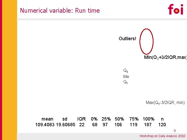
Numerical variable: Run time Outliers! Min(Q 3+3/2 IQR, max) Q 3 Me Q 1 Max(Q 1 -3/2 IQR, min) mean sd IQR 109. 4083 19. 60685 22 0% 25% 50% 68 97 106 75% 100% n 119 187 120 9 Workshop on Data Analysis 2018

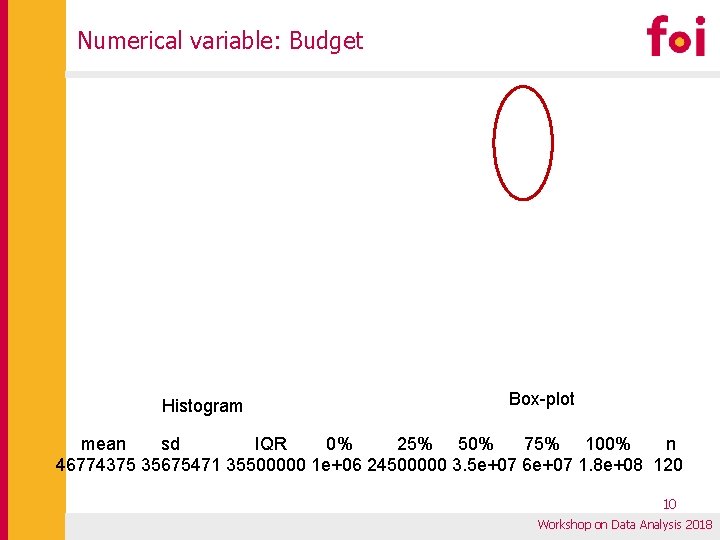
Numerical variable: Budget Histogram Box-plot mean sd IQR 0% 25% 50% 75% 100% n 46774375 35675471 35500000 1 e+06 24500000 3. 5 e+07 6 e+07 1. 8 e+08 120 10 Workshop on Data Analysis 2018

Qualitative variable: Genre Bar chart Pie chart 11 Workshop on Data Analysis 2018

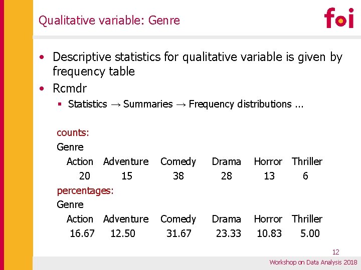
Qualitative variable: Genre • Descriptive statistics for qualitative variable is given by frequency table • Rcmdr § Statistics → Summaries → Frequency distributions. . . counts: Genre Action Adventure 20 15 percentages: Genre Action Adventure 16. 67 12. 50 Comedy 38 Drama 28 Horror Thriller 13 6 Comedy 31. 67 Drama 23. 33 Horror Thriller 10. 83 5. 00 12 Workshop on Data Analysis 2018

Descriptive statistics by group • Statistics can be calculated by factors of qualitative variable • Example: Mean by fators of variable Genre tapply(Movies$Run. Time. . minutes. , list(Genre=Movies$Genre), mean, + na. rm=TRUE) Genre Action Adventure Comedy Drama Horror Thriller 114. 4000 104. 8667 101. 4737 123. 6786 102. 2308 103. 3333 13 Workshop on Data Analysis 2018

Graphs by group: Budget by Genre, boxplot 14 Workshop on Data Analysis 2018

Graphs by group: Run time by Genre, boxplot 15 Workshop on Data Analysis 2018

Random variables • A random event is an event that may or may not occur in a given set of conditions • A random variable is a function of a set of elemental events in a set of real numbers • It is indicated in large letters X, Y, Z. . . • Discrete random variable § A random variable that takes a final or countable infinite set of values • Coutinous random variable § A variable that takes values on interval of real numbers 16 Workshop on Data Analysis 2018

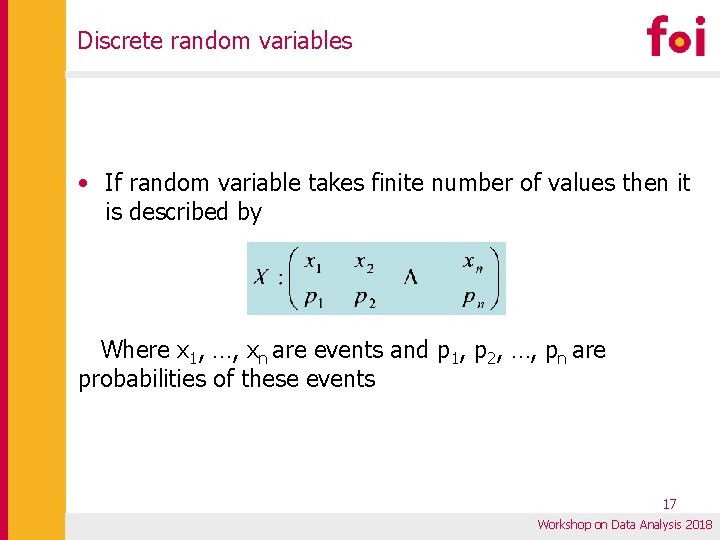
Discrete random variables • If random variable takes finite number of values then it is described by Where x 1, …, xn are events and p 1, p 2, …, pn are probabilities of these events 17 Workshop on Data Analysis 2018

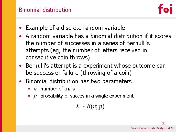
Binomial distribution • Example of a discrete random variable • A random variable has a binomial distribution if it scores the number of successes in a series of Bernulli's attempts (eg, the number of letters received in consecutive coin throws) • Bernulli's attempt is a experiment whose outcome can be success or failure (throwing of a coin) • Binomial distribution has two parameters § n number of trials § p probability of succes in a single experiment 18 Workshop on Data Analysis 2018

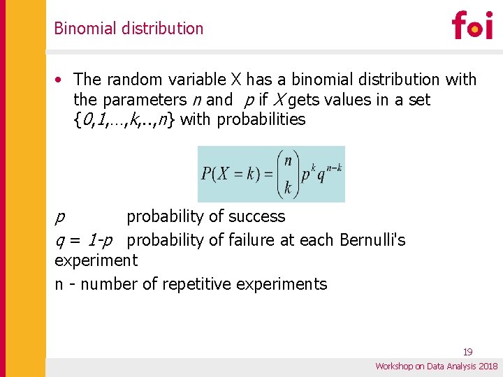
Binomial distribution • The random variable X has a binomial distribution with the parameters n and p if X gets values in a set {0, 1, …, k, . . , n} with probabilities p probability of success q = 1 -p probability of failure at each Bernulli's experiment n - number of repetitive experiments 19 Workshop on Data Analysis 2018

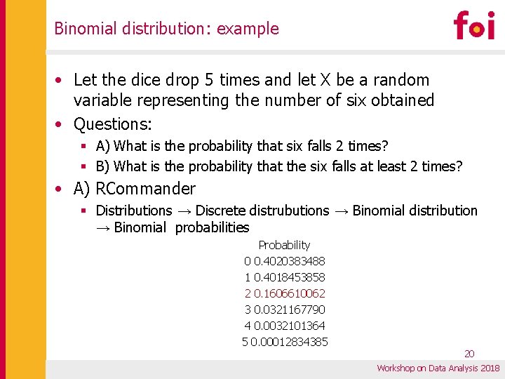
Binomial distribution: example • Let the dice drop 5 times and let X be a random variable representing the number of six obtained • Questions: § A) What is the probability that six falls 2 times? § B) What is the probability that the six falls at least 2 times? • A) RCommander § Distributions → Discrete distrubutions → Binomial distribution → Binomial probabilities Probability 0 0. 4020383488 1 0. 4018453858 2 0. 1606610062 3 0. 0321167790 4 0. 0032101364 5 0. 00012834385 20 Workshop on Data Analysis 2018

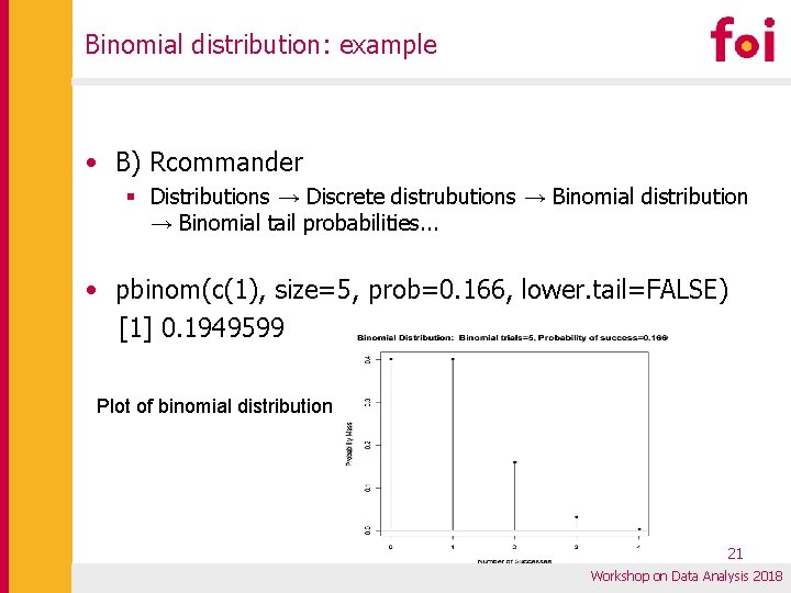
Binomial distribution: example • B) Rcommander § Distributions → Discrete distrubutions → Binomial distribution → Binomial tail probabilities. . . • pbinom(c(1), size=5, prob=0. 166, lower. tail=FALSE) [1] 0. 1949599 Plot of binomial distribution 21 Workshop on Data Analysis 2018

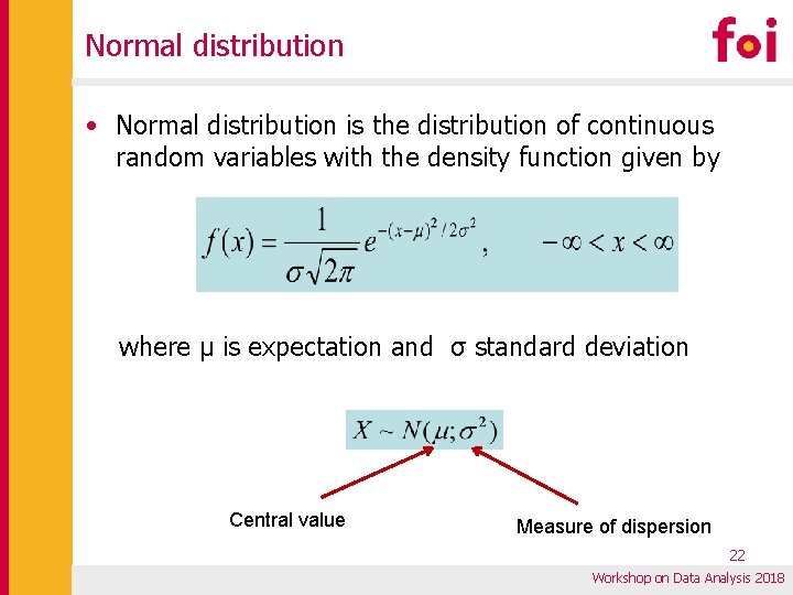
Normal distribution • Normal distribution is the distribution of continuous random variables with the density function given by where µ is expectation and σ standard deviation Central value Measure of dispersion 22 Workshop on Data Analysis 2018

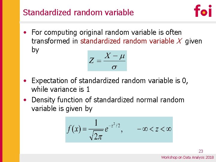
Standardized random variable • For computing original random variable is often transformed in standardized random variable X given by • Expectation of standardized random variable is 0, while variance is 1 • Density function of standardized normal random variable is given by 23 Workshop on Data Analysis 2018

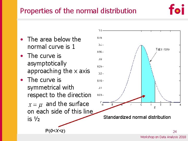
Properties of the normal distribution • The area below the normal curve is 1 • The curve is asymptotically approaching the x axis • The curve is symmetrical with respect to the direction and the surface on each side of this line is ½ P(0<X<z) Standardized normal distribution 24 Workshop on Data Analysis 2018

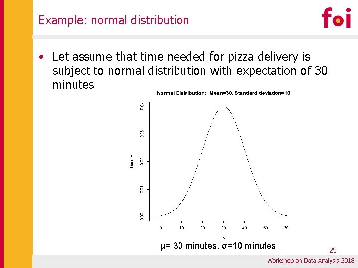
Example: normal distribution • Let assume that time needed for pizza delivery is subject to normal distribution with expectation of 30 minutes μ= 30 minutes, σ=10 minutes 25 Workshop on Data Analysis 2018

Example: normal distribution • Questions § A) Compute the probability that delivery will last more than 45 minuites § B) Compute the time such that 90% of deliveries will last less than it • Answers § A) pnorm(c(45), mean=30, sd=10, lower. tail=FALSE) § 0. 0668072 § R Commander: Distributions → Continuous distributions → Normal distribution → Normal probabilities. . § B) qnorm(c(0. 9), mean=30, sd=10, lower. tail=TRUE) § 42. 81552 § R Commander: Distributions → Continuous distributions → 26 Normal distribution → Normal quantiles. . Workshop on Data Analysis 2018

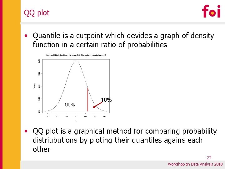
QQ plot • Quantile is a cutpoint which devides a graph of density function in a certain ratio of probabilities 90% 10% • QQ plot is a graphical method for comparing probability distriubutions by ploting their quantiles agains each other 27 Workshop on Data Analysis 2018

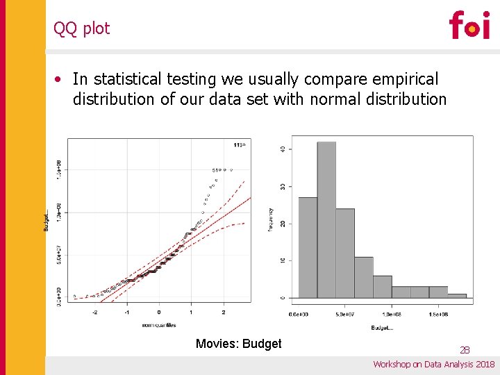
QQ plot • In statistical testing we usually compare empirical distribution of our data set with normal distribution Movies: Budget 28 Workshop on Data Analysis 2018

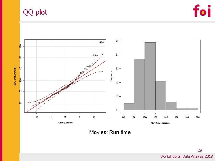
QQ plot Movies: Run time 29 Workshop on Data Analysis 2018

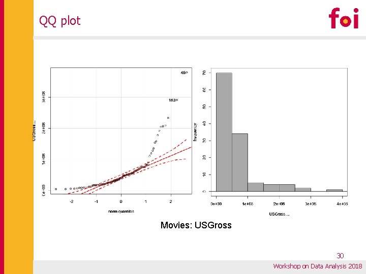
QQ plot Movies: USGross 30 Workshop on Data Analysis 2018

Testing the normality of distribution • Some of statistical tests for testing of normality of distribution are § Chi-square test § Kolmogorov – Smirnov test (KS test) § Shapiro – Wilk’s test • Hypothesis for testing H 0. . . the distribution of the population is subject to the normal distribution H 1. . . the distribution of the population is not subject to the normal distribution 31 Workshop on Data Analysis 2018

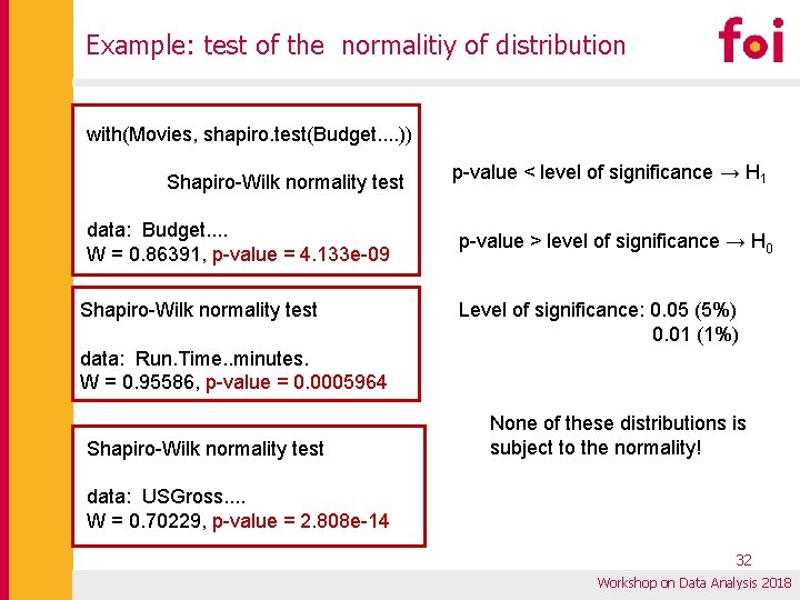
Example: test of the normalitiy of distribution with(Movies, shapiro. test(Budget. . )) Shapiro-Wilk normality test data: Budget. . W = 0. 86391, p-value = 4. 133 e-09 Shapiro-Wilk normality test p-value < level of significance → H 1 p-value > level of significance → H 0 Level of significance: 0. 05 (5%) 0. 01 (1%) data: Run. Time. . minutes. W = 0. 95586, p-value = 0. 0005964 Shapiro-Wilk normality test None of these distributions is subject to the normality! data: USGross. . W = 0. 70229, p-value = 2. 808 e-14 32 Workshop on Data Analysis 2018

Statistical testing • The statistical hypothesis is a claim that refers to the whole population • It is proven on the sample • Hypothesis testing: the procedure or the rule according to which hypothesis is accepted or rejected based on random sample • Statistical tests are divided into parametric and nonparametric • Parametric tests require satisfying conditions on the shape and characteristics of distribution of numeric variables in the population • Nonparametric tests do not require compliance with such conditions 33 Workshop on Data Analysis 2018

Hypothesis and errors in inference • Statistical testing starts by stating null hypothesis (H 0) and alternative hypothesis (H 1) • It is customary to put the claim we want to prove in an alternative hypothesis • Decision about testing is not categorical • Two possible type of errors § Type I error § Incorrect rejection of true null hypothesis § α – level of significance, limit value of probability of rejection of true null hypothesis § Type II error § Retaining a false true null hypothesis § β – limit probability of retaining a false null hypothesis • Power of te test 1 -ß: probability of rejecting a false null hypothesis 34 Workshop on Data Analysis 2018

Decision making • The most comon way to make decision about statistical testing is using p-value • p-value is § empirical value of significance § a probability of rejecting the true null hypothesis calculated by the data from the sample § a measure of the degree of discrediting null hypotheses based on sample data • In testing § If the p-value is greater than the degree of significance α, the null hypothesis is retained § If the p-value is less than the significance level α, the null hypothesis is rejected 35 Workshop on Data Analysis 2018

Testing of means for two populations • Statistical testing can be carried out by § Parametric T – test § Nonparametric tests • We distinguish two types of samples: dependent and independent • Independent samples § the results of observing or measuring in one sample do not depend on the results of observations and measurements in the second sample • Dependent samples • § sample values are obtained by re-observation or by measuring selected variables on the same statistical sample, eg. before and after the experiment (before/after training, before/after treatment) § sample values are given in pairs 36 Workshop on Data Analysis 2018

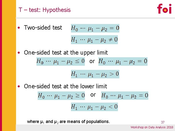
T – test: Hypothesis • Two-sided test • One-sided test at the upper limit or • One-sided test at the lower limit or where μ 1 and μ 2 are means of populations. 37 Workshop on Data Analysis 2018

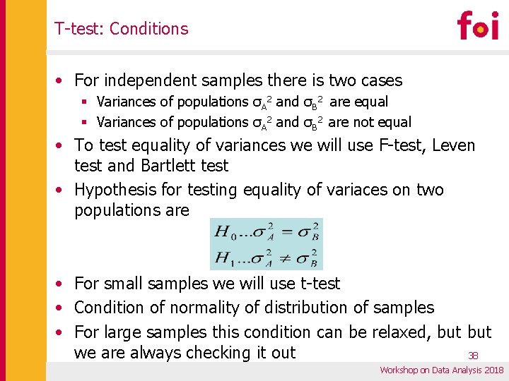
T-test: Conditions • For independent samples there is two cases § Variances of populations σA 2 and σB 2 are equal § Variances of populations σA 2 and σB 2 are not equal • To test equality of variances we will use F-test, Leven test and Bartlett test • Hypothesis for testing equality of variaces on two populations are • For small samples we will use t-test • Condition of normality of distribution of samples • For large samples this condition can be relaxed, but we are always checking it out 38 Workshop on Data Analysis 2018

Similar nonparametric tests • Nonparametric tests we test difference of medains for two populations • Testing of difference of medians for two independent samples § Mann-Whitney-Wilcoxonov test for independet samples (MWW -Test, Rank Sum Test) • Testing of difference of medians for two dependet samples § Sign test § Wilcoxon matched-pairs signed rank test 39 Workshop on Data Analysis 2018

Testing by nonparametric tests • Conditions for nonparametric test are weaker than for parametric tests • The data is represented in the form of signs or rankings • Part of the information is lost • Power of nonparametric tests is lower than power of parametric tests 40 Workshop on Data Analysis 2018

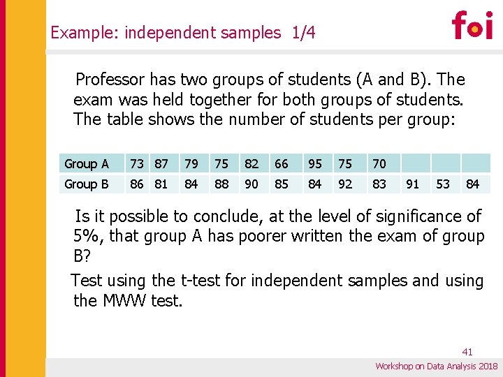
Example: independent samples 1/4 Professor has two groups of students (A and B). The exam was held together for both groups of students. The table shows the number of students per group: Group A 73 87 79 75 82 66 95 75 70 Group B 86 81 84 88 90 85 84 92 83 91 53 84 Is it possible to conclude, at the level of significance of 5%, that group A has poorer written the exam of group B? Test using the t-test for independent samples and using the MWW test. 41 Workshop on Data Analysis 2018

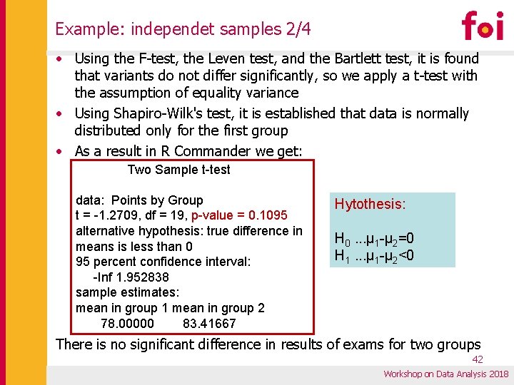
Example: independet samples 2/4 • Using the F-test, the Leven test, and the Bartlett test, it is found that variants do not differ significantly, so we apply a t-test with the assumption of equality variance • Using Shapiro-Wilk's test, it is established that data is normally distributed only for the first group • As a result in R Commander we get: Two Sample t-test data: Points by Group t = -1. 2709, df = 19, p-value = 0. 1095 alternative hypothesis: true difference in means is less than 0 95 percent confidence interval: -Inf 1. 952838 sample estimates: mean in group 1 mean in group 2 78. 00000 83. 41667 Hytothesis: H 0. . . μ 1 -μ 2=0 H 1. . . μ 1 -μ 2<0 There is no significant difference in results of exams for two groups 42 Workshop on Data Analysis 2018

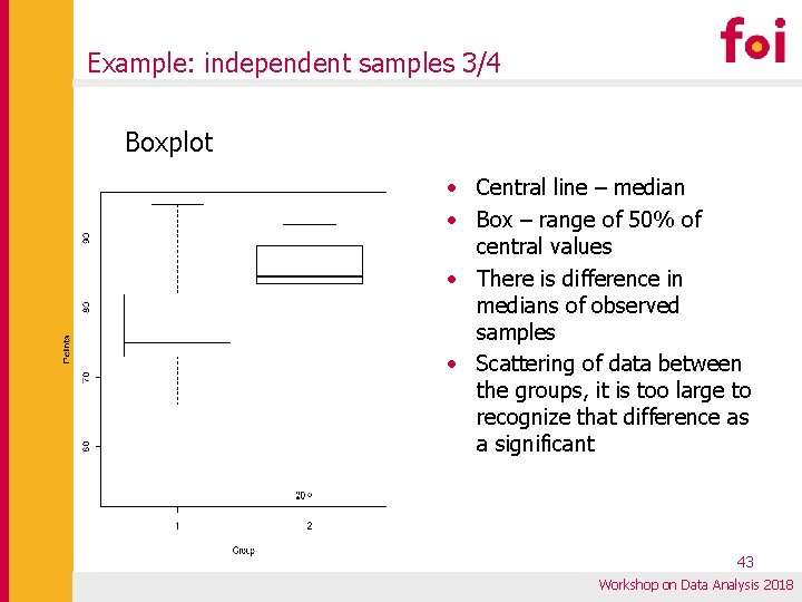
Example: independent samples 3/4 Boxplot • Central line – median • Box – range of 50% of central values • There is difference in medians of observed samples • Scattering of data between the groups, it is too large to recognize that difference as a significant 43 Workshop on Data Analysis 2018

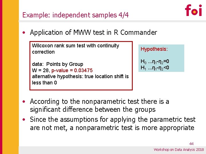
Example: independent samples 4/4 • Application of MWW test in R Commander Wilcoxon rank sum test with continuity correction data: Points by Group W = 28, p-value = 0. 03475 alternative hypothesis: true location shift is less than 0 Hypothesis: H 0. . . η 1 -η 2=0 H 1. . . η 1 -η 2<0 • According to the nonparametric test there is a significant difference between the groups • Since the assumptions for applying the parametric test are not met, a nonparametric test is more appropriate 44 Workshop on Data Analysis 2018

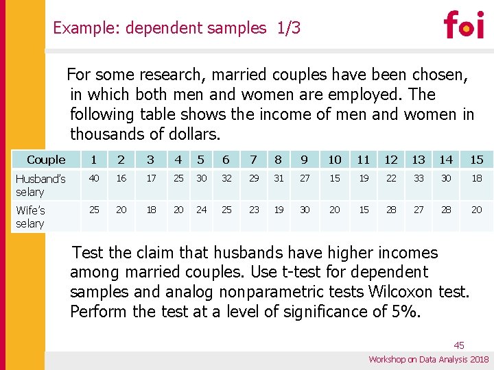
Example: dependent samples 1/3 For some research, married couples have been chosen, in which both men and women are employed. The following table shows the income of men and women in thousands of dollars. Couple 1 2 3 4 5 6 7 8 9 10 11 12 13 14 15 Husband’s selary 40 16 17 25 30 32 29 31 27 15 19 22 33 30 18 Wife’s selary 25 20 18 20 24 25 23 19 30 20 15 28 27 28 20 Test the claim that husbands have higher incomes among married couples. Use t-test for dependent samples and analog nonparametric tests Wilcoxon test. Perform the test at a level of significance of 5%. 45 Workshop on Data Analysis 2018

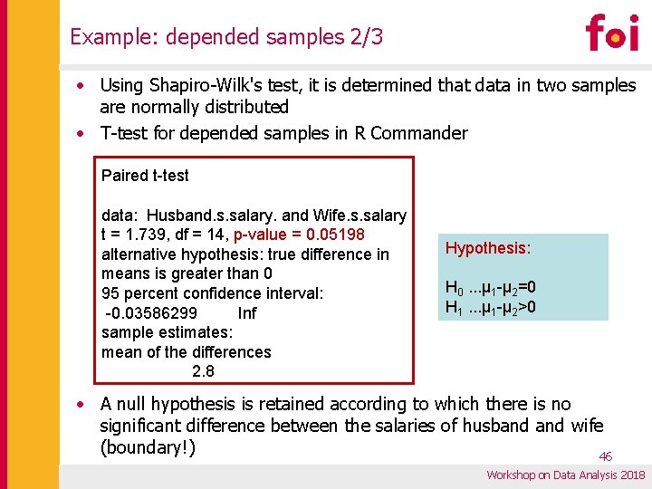
Example: depended samples 2/3 • Using Shapiro-Wilk's test, it is determined that data in two samples are normally distributed • T-test for depended samples in R Commander Paired t-test data: Husband. s. salary. and Wife. s. salary t = 1. 739, df = 14, p-value = 0. 05198 alternative hypothesis: true difference in means is greater than 0 95 percent confidence interval: -0. 03586299 Inf sample estimates: mean of the differences 2. 8 Hypothesis: H 0. . . μ 1 -μ 2=0 H 1. . . μ 1 -μ 2>0 • A null hypothesis is retained according to which there is no significant difference between the salaries of husband wife (boundary!) 46 on Data • Dakle, prihvaća se nulta hipoteza prema kojoj ne. Workshop postoji sig Analysis 2018

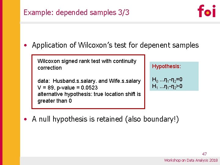
Example: depended samples 3/3 • Application of Wilcoxon’s test for depenent samples Wilcoxon signed rank test with continuity correction data: Husband. s. salary. and Wife. s. salary V = 89, p-value = 0. 0523 alternative hypothesis: true location shift is greater than 0 Hypothesis: H 0. . . η 1 -η 2=0 H 1. . . η 1 -η 2>0 • A null hypothesis is retained (also boundary!) 47 Workshop on Data Analysis 2018

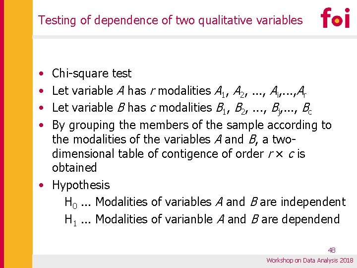
Testing of dependence of two qualitative variables • • Chi-square test Let variable A has r modalities A 1, A 2, . . . , Ai, . . . , Ar Let variable B has c modalities B 1, B 2, . . . , Bj, . . . , Bc By grouping the members of the sample according to the modalities of the variables A and B, a twodimensional table of contigence of order r × c is obtained • Hypothesis H 0. . . Modalities of variables A and B are independent H 1. . . Modalities of varianble A and B are dependend 48 Workshop on Data Analysis 2018

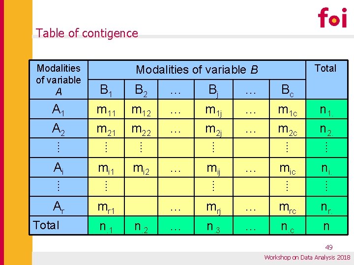
Table of contigence Modalities of variable A B 1 B 2 … Bj … Bc A 1 m 12 … m 1 j … m 1 c n 1. A 2 m 21 m 22 … m 2 j … m 2 c n 2. ⁞ ⁞ ⁞ Ai mi 1 mi 2 mic ni. ⁞ ⁞ Ar mr 1 Total Modalities of variable B n. 1 ⁞ … mij … ⁞ n. 2 … mrj … mrc nr. … n. 3 … n. c n 49 Workshop on Data Analysis 2018

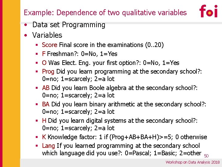
Example: Dependence of two qualitative variables • Data set Programming • Variables § § § § § Score Final score in the examinations (0. . 20) F Freshman? : 0=No, 1=Yes O Was Elect. Eng. your first option? : 0=No, 1=Yes Prog Did you learn programming at the secondary school? : 0=no; 1=scarcely; 2=a lot AB Did you learn Boole algebra at the secondary school? : 0=no; 1=scarcely; 2=a lot BA Did you learn binary arithmetic at the secondary school? : 0=no; 1=scarcely; 2=a lot H Did you learn digital systems at the secondary school? : 0=no; 1=scarcely; 2=a lot K Knowledge factor: 1 if (Prog+AB+BA+H)>=5; 0 otherwise Lang If you learned programming at the secondary school which language did you use? : 0=Pascal; 1=Basic; 2=other 50 Workshop on Data Analysis 2018

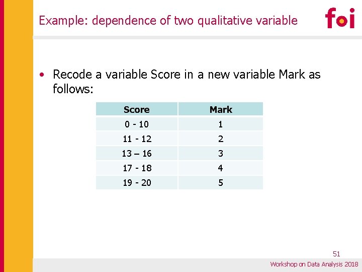
Example: dependence of two qualitative variable • Recode a variable Score in a new variable Mark as follows: Score Mark 0 - 10 1 11 - 12 2 13 – 16 3 17 - 18 4 19 - 20 5 51 Workshop on Data Analysis 2018

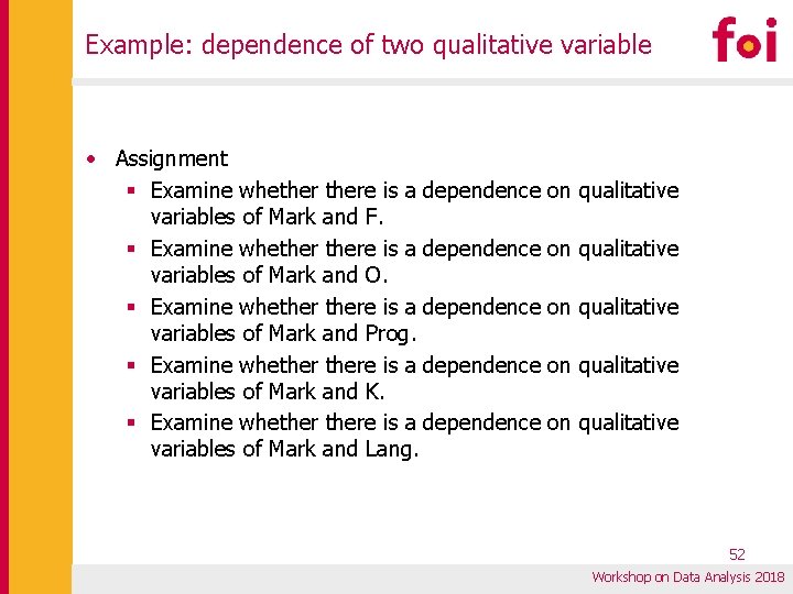
Example: dependence of two qualitative variable • Assignment § Examine whethere is a dependence variables of Mark and F. § Examine whethere is a dependence variables of Mark and O. § Examine whethere is a dependence variables of Mark and Prog. § Examine whethere is a dependence variables of Mark and K. § Examine whethere is a dependence variables of Mark and Lang. on qualitative on qualitative 52 Workshop on Data Analysis 2018

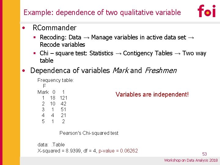
Example: dependence of two qualitative variable • RCommander § Recoding: Data → Manage variables in active data set → Recode variables § Chi – square test: Statistics → Contigency Tables → Two way table • Dependenca of variables Mark and Freshmen Frequency table: F Mark 0 1 1 18 121 2 10 42 3 1 51 4 4 21 5 1 2 Variables are independent! Pearson's Chi-squared test data: . Table X-squared = 8. 9399, df = 4, p-value = 0. 06262 53 Workshop on Data Analysis 2018