Data acquisition and integration Lecture notes Helena Mitasova

Data acquisition and integration Lecture notes Helena Mitasova, NCSU MEAS

Outline Brief overview of what you should already know from the GIS Introductory courses • mapping: data acquisition • coordinate systems and transformations • geospatial data models: raster, vector • raster-vector conversions and resampling • geospatial formats and conversions • data repositories, interpreting metadata

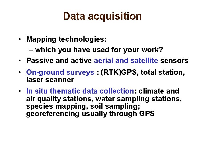
Data acquisition • Mapping technologies: – which you have used for your work? • Passive and active aerial and satellite sensors • On-ground surveys : (RTK)GPS, total station, laser scanner • In situ thematic data collection: climate and air quality stations, water sampling stations, species mapping, soil sampling; georeferencing usually through GPS

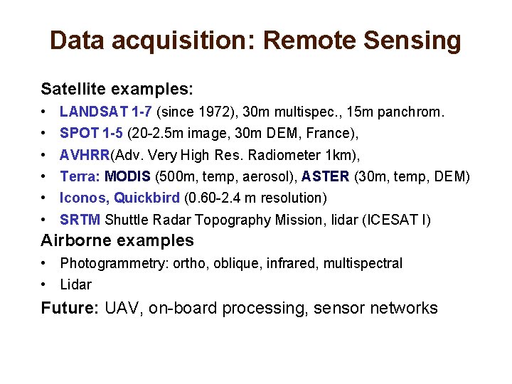
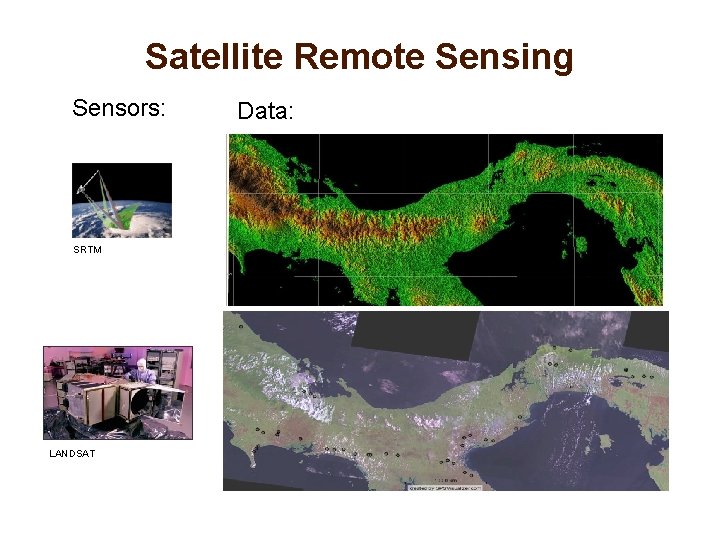
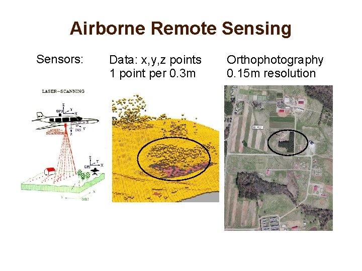
Data acquisition: Remote Sensing Satellite examples: • • • LANDSAT 1 -7 (since 1972), 30 m multispec. , 15 m panchrom. SPOT 1 -5 (20 -2. 5 m image, 30 m DEM, France), AVHRR(Adv. Very High Res. Radiometer 1 km), Terra: MODIS (500 m, temp, aerosol), ASTER (30 m, temp, DEM) Iconos, Quickbird (0. 60 -2. 4 m resolution) SRTM Shuttle Radar Topography Mission, lidar (ICESAT I) Airborne examples • Photogrammetry: ortho, oblique, infrared, multispectral • Lidar Future: UAV, on-board processing, sensor networks

Satellite Remote Sensing Sensors: SRTM LANDSAT Data:

Airborne Remote Sensing Sensors: Data: x, y, z points 1 point per 0. 3 m Orthophotography 0. 15 m resolution

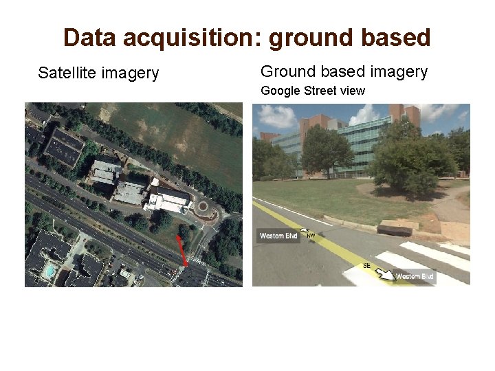
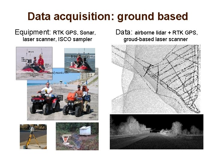
Data acquisition: ground-based • GPS, RTK-GPS • terrestrial photogrammetry static and mobile • laser scanners static or mobile on cars/robots • discipline specific monitoring and sampling stations (econet station, ISCO sampler) • Products: georeferenced points with attributes or “streetview” imagery

Data acquisition: ground based Satellite imagery Ground based imagery Google Street view

Data acquisition: ground based Equipment: RTK GPS, Sonar, laser scanner, ISCO sampler Data: airborne lidar + RTK GPS, groud-based laser scanner

From mapping to GIS • georeferencing (real-time during mapping with GPS) • feature or theme extraction • building GIS data model representation (raster or vector with attribute database) Mapped data (imagery or points) are transformed into georeferenced, discrete representations of landscape features

Georeferencing • Georeferenced data: location on Earth is represented in a Coordinate Referenced System • MANY coordinate systems exist, they evolve over time as accuracy of the Earth measurements improves

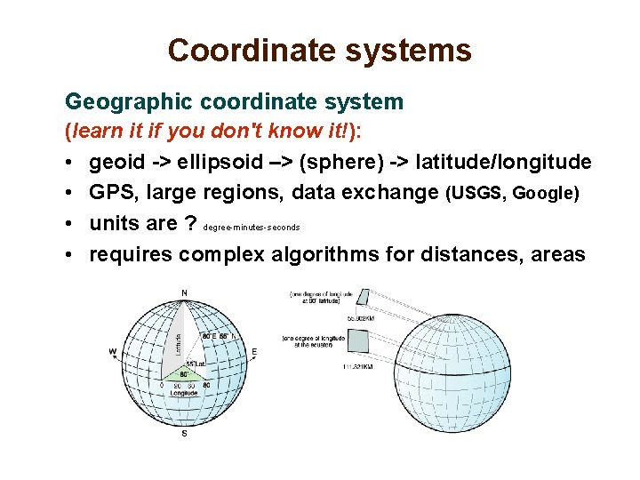
Coordinate systems Geographic coordinate system (learn it if you don't know it!): • geoid -> ellipsoid –> (sphere) -> latitude/longitude • GPS, large regions, data exchange (USGS, Google) • units are ? degree-minutes-seconds • requires complex algorithms for distances, areas

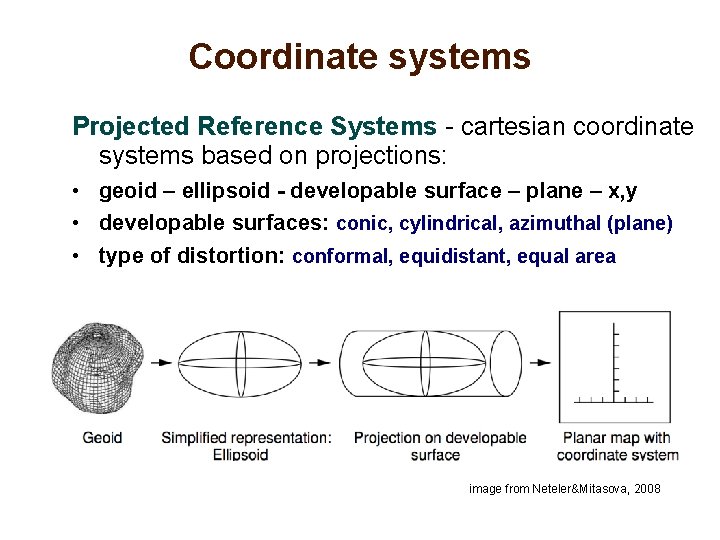
Coordinate systems Projected Reference Systems - cartesian coordinate systems based on projections: • geoid – ellipsoid - developable surface – plane – x, y • developable surfaces: conic, cylindrical, azimuthal (plane) • type of distortion: conformal, equidistant, equal area & image from Neteler&Mitasova, 2008

Cartographic Projections To learn more about Projected Reference Systems please read: www. progonos. com/furuti/Map. Proj/Normal/TOC/cart. TOC. html excellent, easy to understand material about projections and map properties with lots of graphics and mathematical foundations, and fun to read see also links to references in this document

National and state systems National/State Coordinate systems defined by: • Reference spheroid/geoid and datum • Vertical datum • Projection Goal was to minimize distortions on maps that were used to measure distances and areas – less important now when distances and areas are computed directly from data

National and state systems Reference geoid and datum: • North American: Clarke 1866 - NAD 27, Grs 80 - NAD 83 • World geodetic system WGS 84 • Vertical datums: NGVD 29 - National Geodetic Vertical Datum 1929, NAVD 88 – North american Vertical Datum 1988 Projections • Lambert Conformal Conic (LCC): states in US • Universal Transverse Mercator (UTM): USGS, military • Albers Equal Area (conic): USGS national map

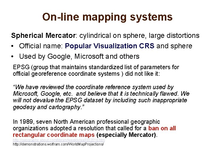
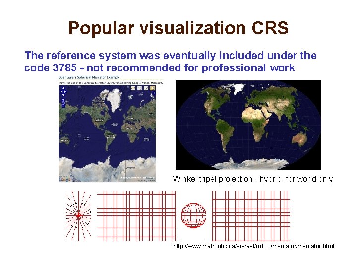
On-line mapping systems Spherical Mercator: cylindrical on sphere, large distortions • Official name: Popular Visualization CRS and sphere • Used by Google, Microsoft and others EPSG (group that maintains standardized list of parameters for official georeference coordinate systems ) did not like it: “We have reviewed the coordinate reference system used by Microsoft, Google, etc. and believe that it is technically flawed. We will not devalue the EPSG dataset by including such inappropriate geodesy and cartography. ” In 1989, seven North American professional geographic organizations adopted a resolution that called for a ban on all rectangular coordinate maps (especially Mercator). http: //geography. about. com/library/weekly/aa 030201 b. htm http: //demonstrations. wolfram. com/World. Map. Projections/

Popular visualization CRS The reference system was eventually included under the code 3785 - not recommended for professional work Winkel tripel projection - hybrid, for world only http: //www. math. ubc. ca/~israel/m 103/mercator. html

Coordinate systems in GIS Representation of coordinate systems in GIS • Metadata file • ESRI PRJ file • EPSG codes provided by OGP - Int. Org. of Oil and Gas Producers Surveying and Positioning Committee, formerly EPSG – european petroleum survey group • http: //mapserver. gis. umn. edu/docs/faq/epsg_codes Vertical datum support often missing in GIS – specialized tools

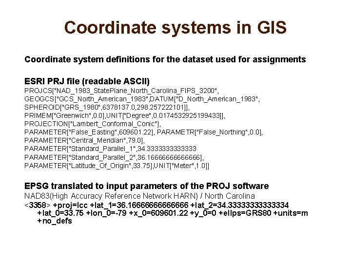
Coordinate systems in GIS Coordinate system definitions for the dataset used for assignments ESRI PRJ file (readable ASCII) PROJCS["NAD_1983_State. Plane_North_Carolina_FIPS_3200", GEOGCS["GCS_North_American_1983", DATUM["D_North_American_1983", SPHEROID["GRS_1980", 6378137. 0, 298. 257222101]], PRIMEM["Greenwich", 0. 0], UNIT["Degree", 0. 0174532925199433]], PROJECTION["Lambert_Conformal_Conic"], PARAMETER["False_Easting", 609601. 22], PARAMETR["False_Northing", 0. 0], PARAMETER["Central_Meridian", 79. 0], PARAMETER["Standard_Parallel_1", 34. 3333333 PARAMETER["Standard_Parallel_2", 36. 16666666], PARAMETER["Latitude_Of_Origin", 33. 75], UNIT["Meter", 1. 0]] EPSG translated to input parameters of the PROJ software NAD 83(High Accuracy Reference Network HARN) / North Carolina <3358> +proj=lcc +lat_1=36. 16666666 +lat_2=34. 33333334 +lat_0=33. 75 +lon_0=-79 +x_0=609601. 22 +y_0=0 +ellps=GRS 80 +units=m +no_defs

Coordinate transformations Data often come in different coordinate systems: • USGS, federal agencies: Geographic coordinates, Albers equal area, UTM • State agencies: State Plane • Older data may have different datums (NAD 27, NAD 83) Coordinate transformations • x, y -> longitude, latitude -> x’, y’ • on-fly transformation may be time consuming, especially for raster : resampling/reinterpolation to regular grid is required

Geospatial data models Mapped, georeferenced data are transformed into discrete GIS representations using • raster (regular grid) • vector (feature: point, line, area/polygon) geospatial data models

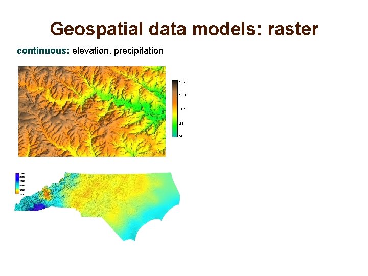
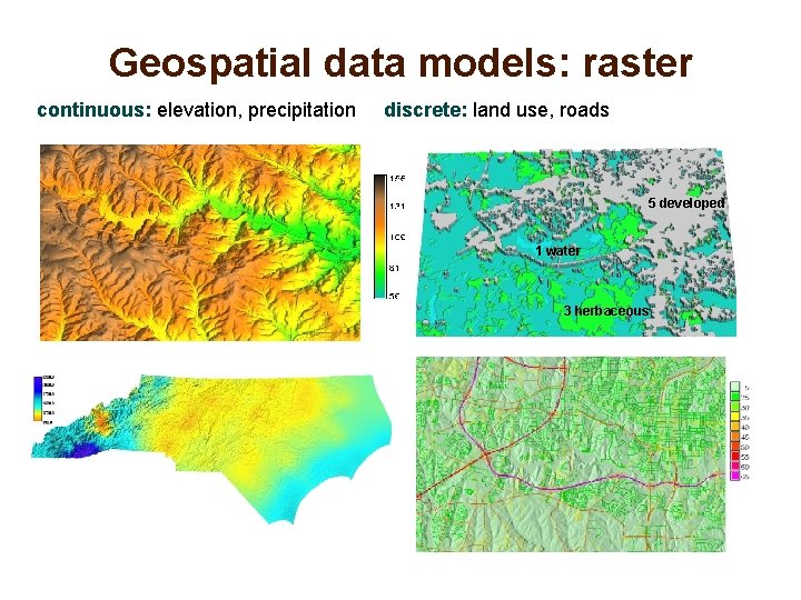
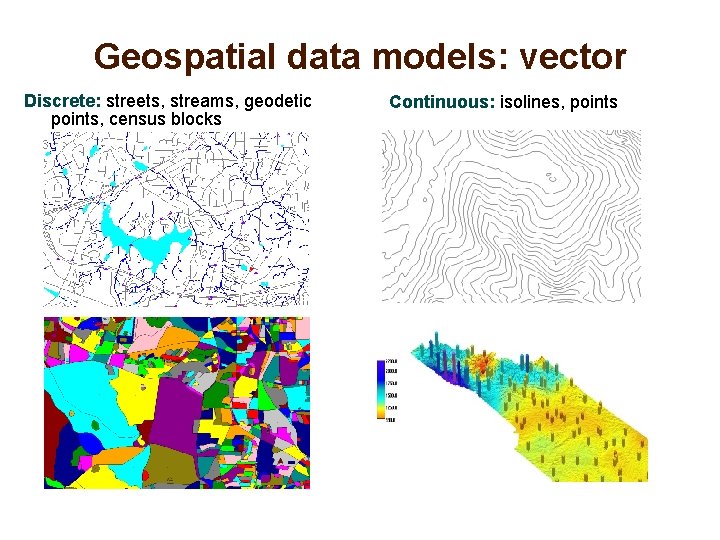
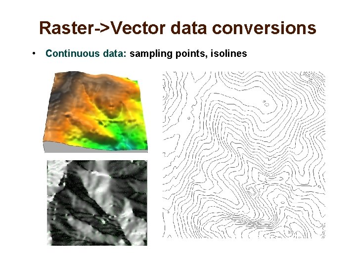
Geospatial data models Two different types of objects/phenomena – continuous fields: w=f(x, y), w=f(x, y, z) each point in space is assigned a distinct value, change between two neighboring points is relatively small: elevation, precipitation represented by raster data model, but vector model is also used: meshes, TIN, isolines or points. – discrete objects/features: lines, points or areas with attributes represented by vector data model as geometry(shape) with attribute table or object based (geodatabase); raster representation is also used : roads, streams, census blocks, land use, schools

Geospatial data models: raster continuous: elevation, precipitation

Geospatial data models: raster continuous: elevation, precipitation discrete: land use, roads 5 developed 1 water 3 herbaceous

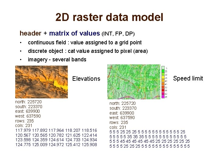
2 D raster data model header + matrix of values (INT, FP, DP) • continuous field : value assigned to a grid point • discrete object : cat value assigned to pixel (area) • imagery - several bands Elevations north: 225720 south: 223370 east: 639900 west: 637590 rows: 235 cols: 231 117. 979 117. 892 117. 964 118. 207 118. 516 120. 567 120. 565 120. 782 121. 625 122. 414 123. 598 124. 359 124. 614 124. 733 124. 934 124. 775 125. 009 124. 972 125. 412 125. 908 Speed limit north: 225720 south: 223370 east: 639900 west: 637590 rows: 235 cols: 231 5 5 5 25 25 25 5 5 5 25 5 5 35 35 35 5 5 5 45 45 45 25 25 25 5 5 5 5

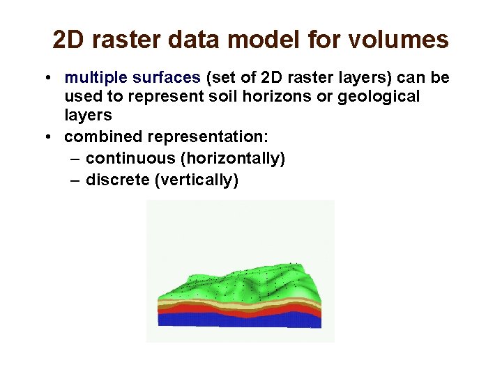
2 D raster data model for volumes • multiple surfaces (set of 2 D raster layers) can be used to represent soil horizons or geological layers • combined representation: – continuous (horizontally) – discrete (vertically)

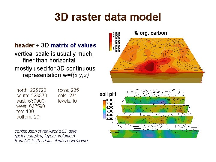
3 D raster data model % org. carbon header + 3 D matrix of values vertical scale is usually much finer than horizontal mostly used for 3 D continuous representation w=f(x, y, z) north: 225720 south: 223370 east: 639900 west: 637590 top: 130 bottom: 20 rows: 235 cols: 231 levels: 10 contribution of real-world 3 D data (point samples, layers, volumes) from NC to the dataset will be welcome soil p. H

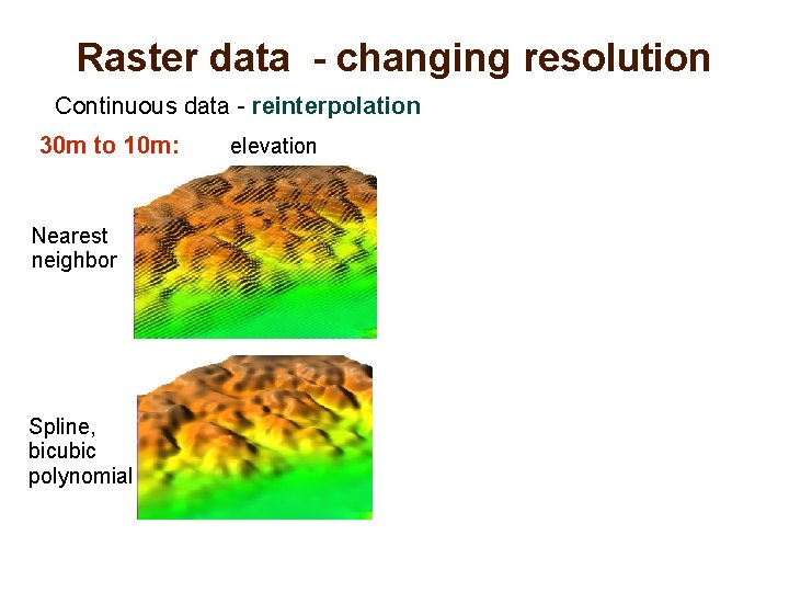
Raster data - changing resolution Continuous data - reinterpolation 30 m to 10 m: Nearest neighbor Spline, bicubic polynomial elevation

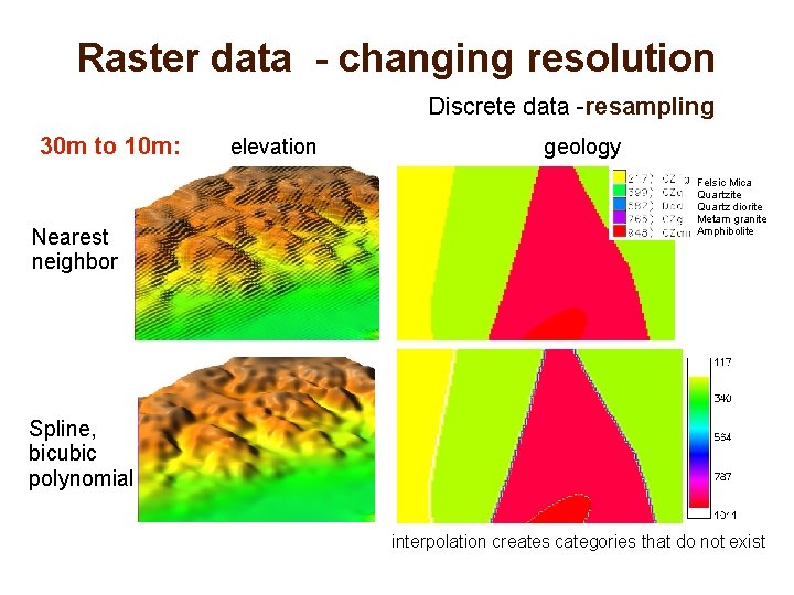
Raster data - changing resolution Discrete data -resampling 30 m to 10 m: Nearest neighbor elevation geology Felsic Mica Quartzite Quartz diorite Metam granite Amphibolite Spline, bicubic polynomial interpolation creates categories that do not exist

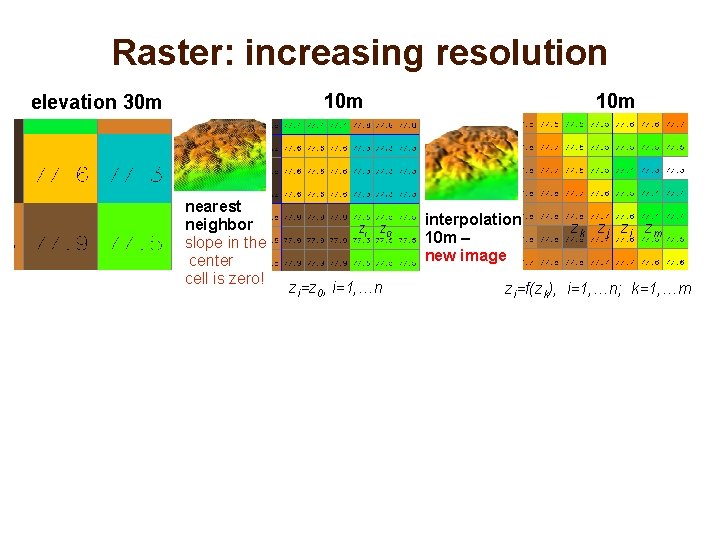
Raster: increasing resolution 10 m elevation 30 m nearest neighbor slope in the center cell is zero! zi z 0 zi=z 0, i=1, …n 10 m interpolation 10 m – new image zk zj zi zm zi=f(zk), i=1, …n; k=1, …m

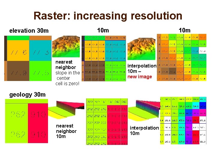
Raster: increasing resolution 10 m elevation 30 m nearest neighbor slope in the center cell is zero! 10 m interpolation 10 m – new image geology 30 m nearest neighbor 10 m interpolation 10 m

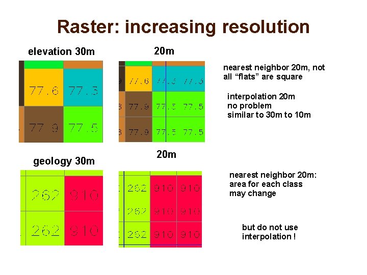
Raster: increasing resolution elevation 30 m 20 m nearest neighbor 20 m, not all “flats” are square interpolation 20 m no problem similar to 30 m to 10 m geology 30 m 20 m nearest neighbor 20 m: area for each class may change but do not use interpolation !

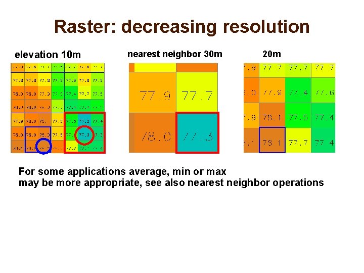
Raster: decreasing resolution elevation 10 m nearest neighbor 30 m 20 m For some applications average, min or max may be more appropriate, see also nearest neighbor operations

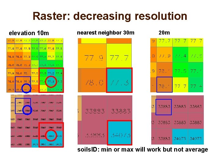
Raster: decreasing resolution elevation 10 m nearest neighbor 30 m 20 m soils. ID: min or max will work but not average

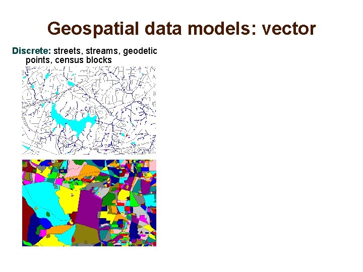
Geospatial data models: vector Discrete: streets, streams, geodetic points, census blocks

Geospatial data models: vector Discrete: streets, streams, geodetic points, census blocks Continuous: isolines, points

Geospatial data models: vector data model - geometry: • [x, y, (z)] points representing points, lines, areas • topology: nodes, vertices, centroids, line, polyline, boundary, polygon • 3 D vector data: face, kernel volume points, lines areas

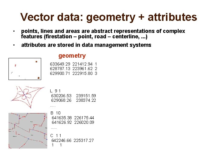
Vector data: geometry + attributes • points, lines and areas are abstract representations of complex features (firestation – point, road – centerline, . . . ) • attributes are stored in data management systems geometry 633649. 29 221412. 94 1 628787. 13 223961. 62 2 629900. 71 222915. 80 3 L 91 630206. 53 629068. 26 …. 239151. 59 238374. 22 B 10 641635. 38 226175. 44 641626. 92 226020. 09. . . C 11 642246. 66 225317. 27 1 1

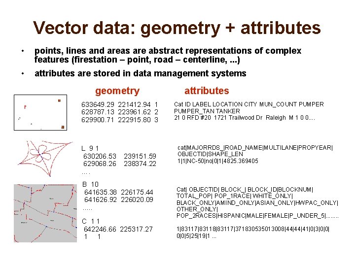
Vector data: geometry + attributes • points, lines and areas are abstract representations of complex features (firestation – point, road – centerline, . . . ) • attributes are stored in data management systems geometry 633649. 29 221412. 94 1 628787. 13 223961. 62 2 629900. 71 222915. 80 3 L 91 630206. 53 629068. 26 …. 239151. 59 238374. 22 B 10 641635. 38 226175. 44 641626. 92 226020. 09. . . C 11 642246. 66 225317. 27 1 1 attributes Cat ID LABEL LOCATION CITY MUN_COUNT PUMPER_TAN TANKER 21 0 RFD #20 1721 Trailwood Dr Raleigh M 1 0 0. . cat|MAJORRDS_|ROAD_NAME|MULTILANE|PROPYEAR| OBJECTID|SHAPE_LEN 1|1|NC-50|no|0|1|4825. 369405 Cat| OBJECTID| BLOCK_ID|BLOCKNUM| TOTAL_POP| POP_1 RACE| WHITE_ONLY| BLACK_ONLY|AMIND_ONLY|ASIAN_ONLY|HWPAC_ONLY| OTHER_ONLY| POP_2 RACES|HISPANIC|MALE|FEMALE|P_UNDER_5|. . . . 1|83117|83118|83117|371830535013008|44|44|41|0|3|0|0|5|25|19|1. . .

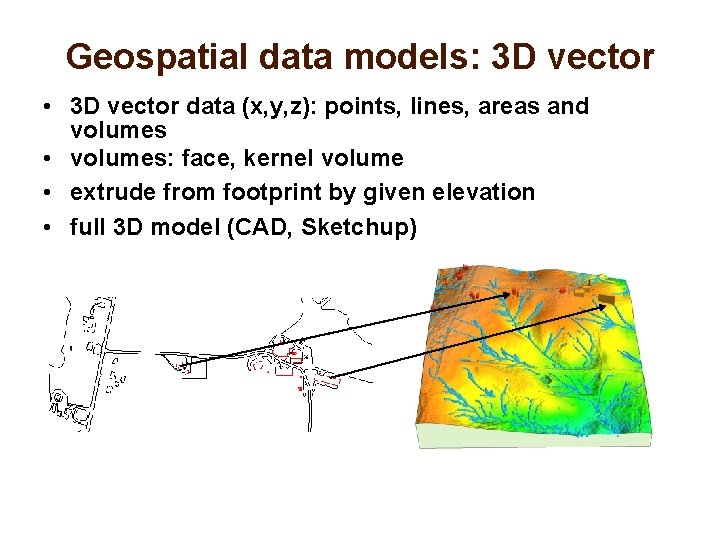
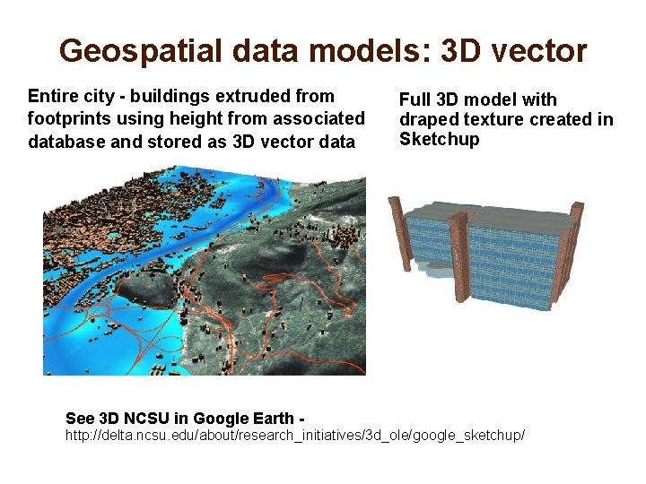
Geospatial data models: 3 D vector • 3 D vector data (x, y, z): points, lines, areas and volumes • volumes: face, kernel volume • extrude from footprint by given elevation • full 3 D model (CAD, Sketchup)

Geospatial data models: 3 D vector Entire city - buildings extruded from footprints using height from associated database and stored as 3 D vector data Full 3 D model with draped texture created in Sketchup See 3 D NCSU in Google Earth http: //delta. ncsu. edu/about/research_initiatives/3 d_ole/google_sketchup/

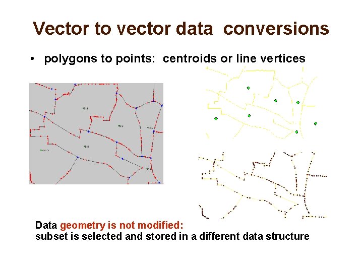
Vector to vector data conversions • polygons to points: centroids or line vertices Data geometry is not modified: subset is selected and stored in a different data structure

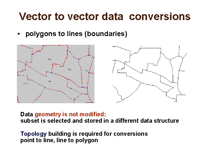
Vector to vector data conversions • polygons to lines (boundaries) Data geometry is not modified: subset is selected and stored in a different data structure Topology building is required for conversions point to line, line to polygon

Vector to vector data conversions Generalization (downscaling) - geometry is simplified • roads, streams, contours, building footprints, urban areas, coastlines • line to simplified line • polygon (building footprint, urban area) to point symbol Both data geometry and type can be modified Needs to be considered when combining local, state and national scale data Streams: 1: 2000 local, 1: 24000 topomap, 1: 1 mil national

Conversions between data models Vector to Raster to Vector

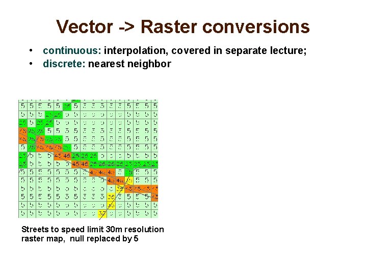
Vector -> Raster conversions • continuous: interpolation, covered in separate lecture; • discrete: nearest neighbor Streets to speed limit 30 m resolution raster map, null replaced by 5

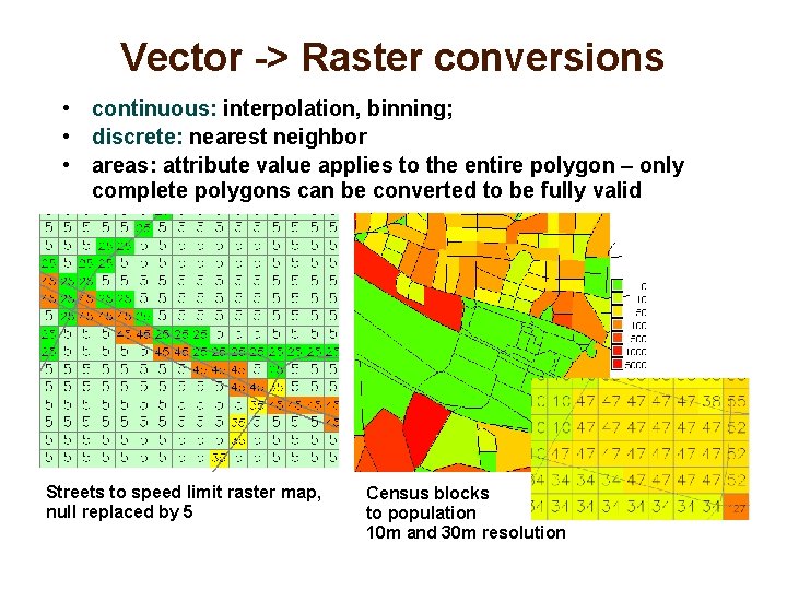
Vector -> Raster conversions • continuous: interpolation, binning; • discrete: nearest neighbor • areas: attribute value applies to the entire polygon – only complete polygons can be converted to be fully valid Streets to speed limit raster map, null replaced by 5 Census blocks to population 10 m and 30 m resolution

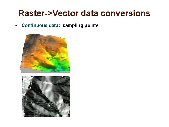
Raster->Vector data conversions • Continuous data: sampling points

Raster->Vector data conversions • Continuous data: sampling points, isolines

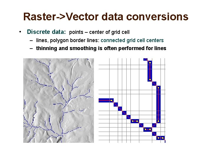
Raster->Vector data conversions • Discrete data: points – center of grid cell – lines, polygon border lines: connected grid cell centers – thinning and smoothing is often performed for lines

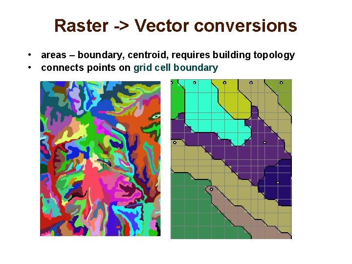
Raster -> Vector conversions • areas – boundary, centroid, requires building topology • connects points on grid cell boundary

Common geospatial data formats Raster ? Vector ?

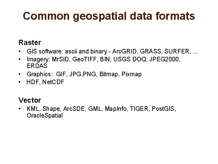
Common geospatial data formats Raster • GIS software: ascii and binary - Arc. GRID, GRASS, SURFER, . . . • Imagery: Mr. SID, Geo. TIFF, BIN, USGS DOQ, JPEG 2000, ERDAS • Graphics: GIF, JPG, PNG, Bitmap, Pixmap • HDF, Net. CDF Vector • KML, Shape, Arc. SDE, GML, Map. Info, TIGER, Post. GIS, Oracle. Spatial

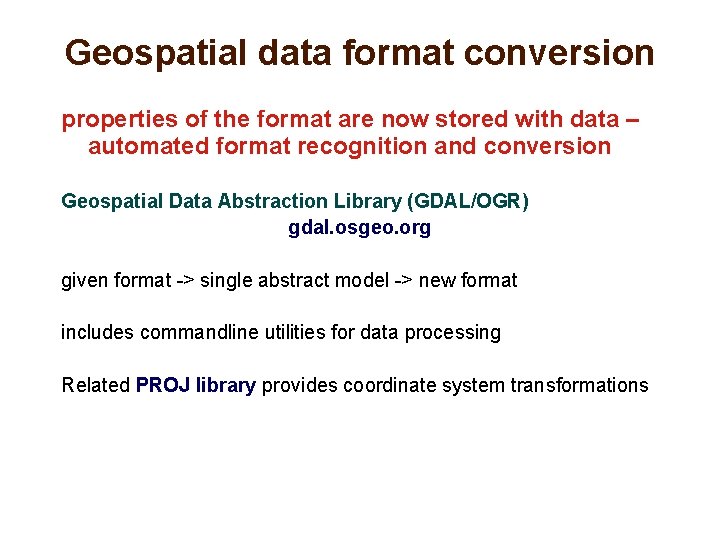
Geospatial data format conversion properties of the format are now stored with data – automated format recognition and conversion Geospatial Data Abstraction Library (GDAL/OGR) gdal. osgeo. org given format -> single abstract model -> new format includes commandline utilities for data processing Related PROJ library provides coordinate system transformations

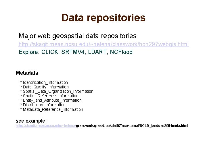
Data repositories Major web geospatial data repositories http: //skagit. meas. ncsu. edu/~helena/classwork/hon 297 webgis. html Explore: CLICK, SRTMV 4, LDART, NCFlood Metadata * Identification_Information * Data_Quality_Information * Spatial_Data_Organization_Information * Spatial_Reference_Information * Entity_and_Attribute_Information * Distribution_Information * Metadata_Reference_Information see example: http: //skagit. meas. ncsu. edu/~helena/grasswork/grassbookdat 07/ncexternal/NCLD_landuse 2001 meta. html

Summary and references • Data acquisition – Bolstad: GIS fundamentals, Ch. 5, – Chang Ch. 5. 2, 6 • Coordinate systems and transformations, georeferencing mandatory reading: www. progonos. com/furuti/Map. Proj/Normal/TOC/cart. TOC. html • Data models: raster / vector, continuous / discrete – Chang Ch. 3, 4, 5, Neteler Ch. 2. 1, 4. 1. 1 and 4. 2. 1 • links on the relevant slides

Summary and References • Data models: raster / vector, continuous / discrete – Chang Ch. 3, 4, 5, Neteler Ch. 2. 1, 4. 1. 1 and 4. 2. 1 • Raster-vector conversions and resampling – Chang 5. 5, Neteler Ch 5. 3, 6. 7 • Geospatial data formats, conversions – Chang Ch 3, 4, 5. 2 -4, Neteler Ch. 4 • Data repositories