Customer choice Customer choice Outline The binary logit

Customer choice

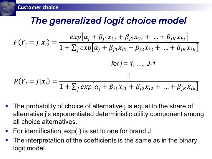
Customer choice Outline § The binary logit choice model Illustration □ Specification of the binary logit choice model □ Interpreting the results of binary logit choice models □ Office Star example □ § The generalized logit choice model Specification of the generalized logit choice model □ Interpreting the results of generalized logit choice models □ Office Star example □

Customer choice Learning goals § Understand the basic idea of the binary logit choice model § Know how to specify a binary choice model and interpret the results § Understand the basic idea of the generalized logit choice model § Know how to specify a generalized logit choice model and interpret the results

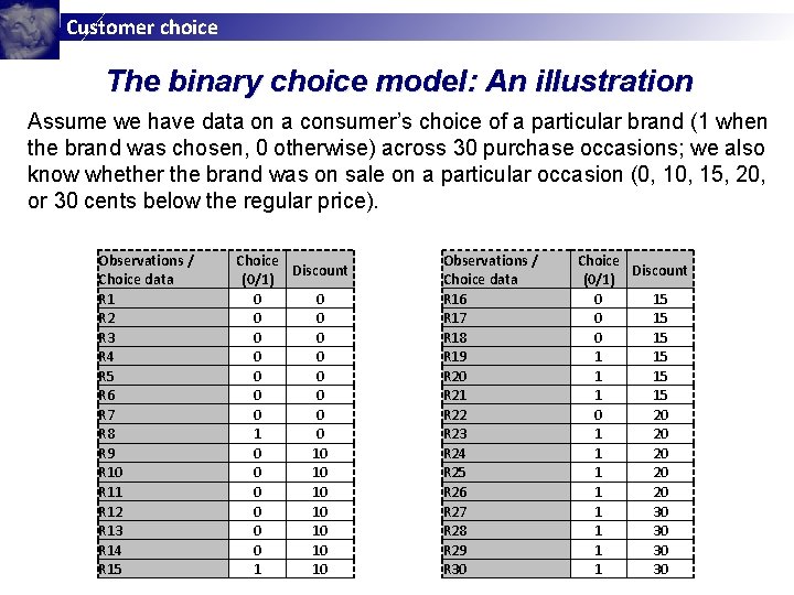
Customer choice The binary choice model: An illustration Assume we have data on a consumer’s choice of a particular brand (1 when the brand was chosen, 0 otherwise) across 30 purchase occasions; we also know whether the brand was on sale on a particular occasion (0, 15, 20, or 30 cents below the regular price). Observations / Choice data R 1 R 2 R 3 R 4 R 5 R 6 R 7 R 8 R 9 R 10 R 11 R 12 R 13 R 14 R 15 Choice Discount (0/1) 0 0 0 0 1 0 0 10 0 10 1 10 Observations / Choice data R 16 R 17 R 18 R 19 R 20 R 21 R 22 R 23 R 24 R 25 R 26 R 27 R 28 R 29 R 30 Choice Discount (0/1) 0 15 1 15 0 20 1 20 1 30

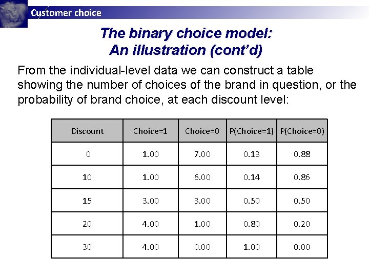
Customer choice The binary choice model: An illustration (cont’d) From the individual-level data we can construct a table showing the number of choices of the brand in question, or the probability of brand choice, at each discount level: Discount Choice=1 Choice=0 P(Choice=1) P(Choice=0) 0 1. 00 7. 00 0. 13 0. 88 10 1. 00 6. 00 0. 14 0. 86 15 3. 00 0. 50 20 4. 00 1. 00 0. 80 0. 20 30 4. 00 0. 00 1. 00 0. 00

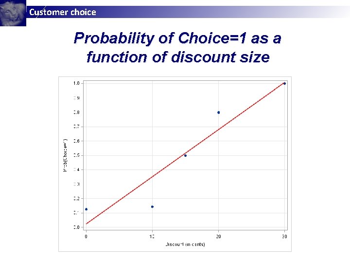
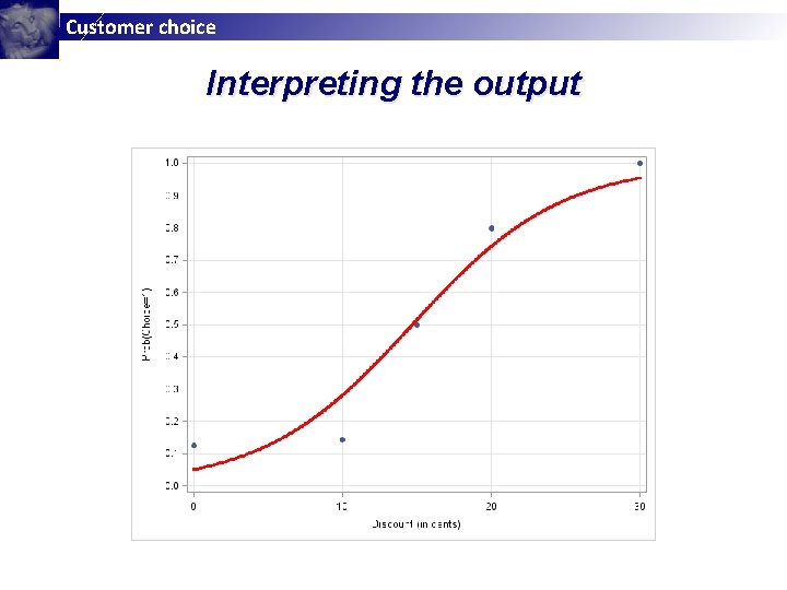
Customer choice Probability of Choice=1 as a function of discount size

Customer choice The binary choice model: An illustration (cont’d) § Two issues: If the discount is larger than 30 cents, the model predicts a probability greater than 1. □ We can only compute a probability if we have multiple 0/1 observations for each level of discount. □ § Solution: Choose an S-shaped curve that restricts the probability of choice to the interval of 0 to 1. □ Assume that the 0/1 variable is a crude measure of an underlying probability of choice. □

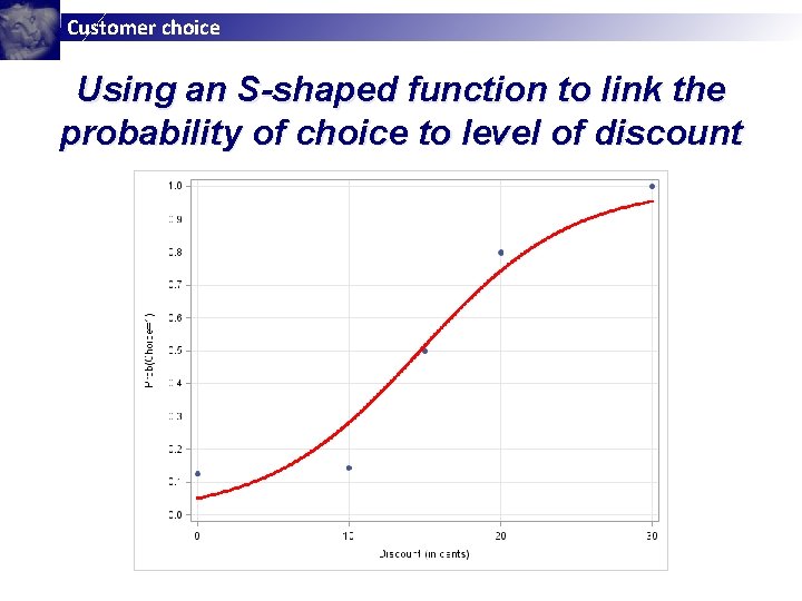
Customer choice Using an S-shaped function to link the probability of choice to level of discount

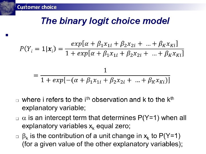
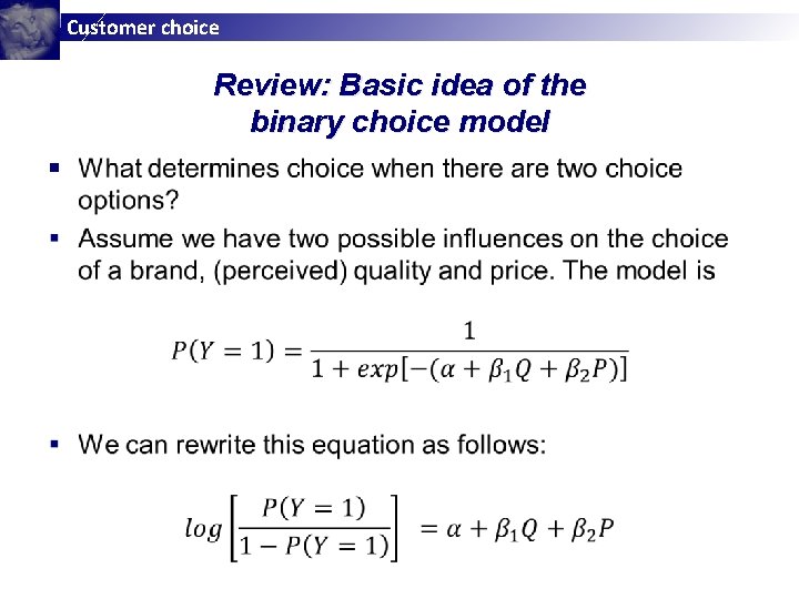
Customer choice The binary logit choice model §

Customer choice How to calculate P [ Y=1 ] ? §

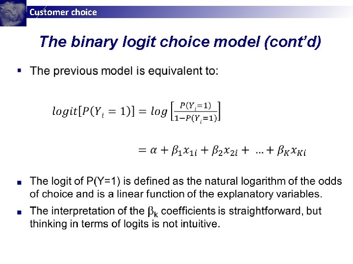
Customer choice The binary logit choice model (cont’d)

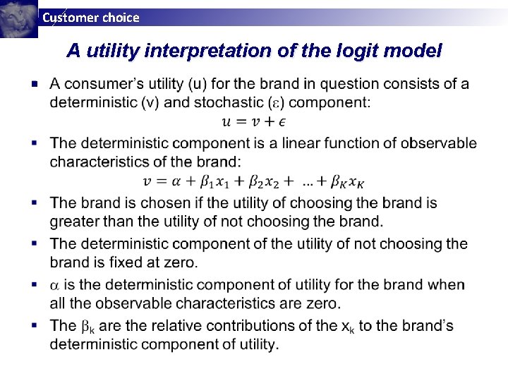
Customer choice A utility interpretation of the logit model §

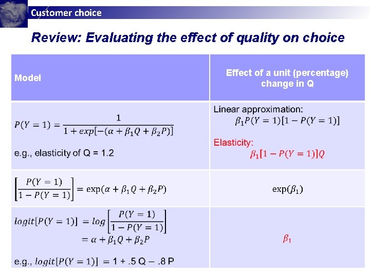
Customer choice Improving the interpretability of binary choice models §

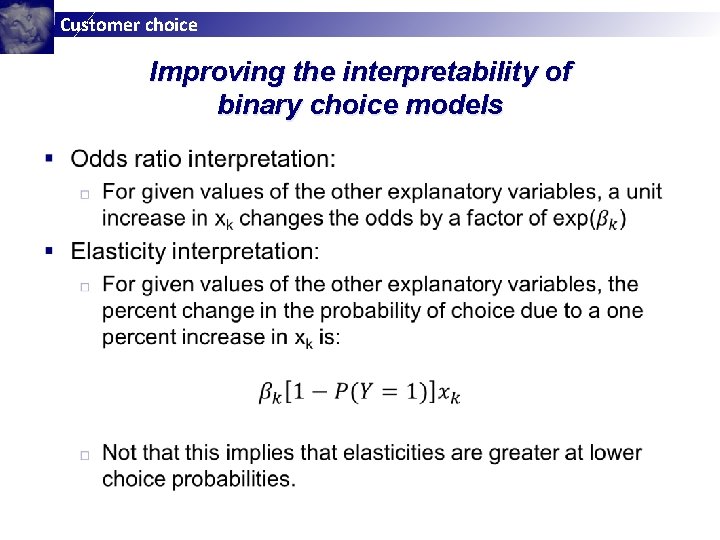
Customer choice Improving the interpretability of binary choice models

Customer choice Illustrative example: Estimation results Coefficient Estimates [segment 1] Coefficient estimates of the Choice model. Coefficients in bold are statistically significant. Variables / Coefficient estimates Discount Const-1 Baseline Coefficient estimates Standard deviation t-statistic 0. 199905 -2. 93693 0. 075153 1. 138345 n/a 2. 659987 -2. 58 n/a Elasticities [segment 1] Elasticities of coefficients. Elasticities of Discount Response Dummy (No Choice) 0. 931691 0 -0. 71248 0

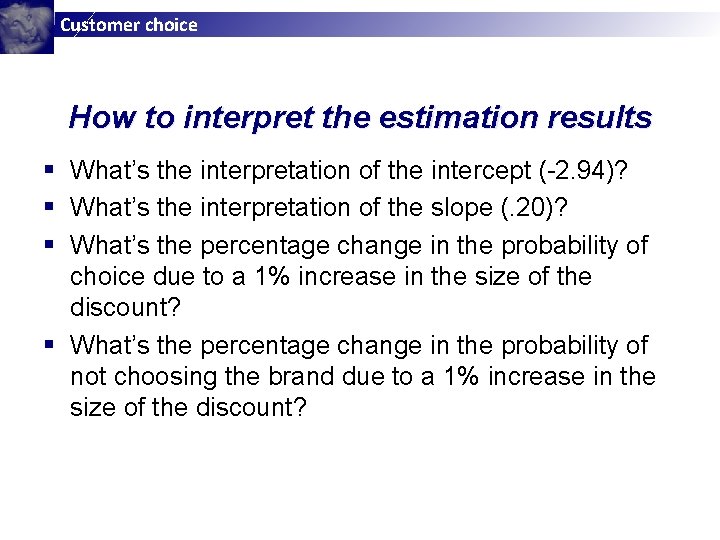
Customer choice How to interpret the estimation results § What’s the interpretation of the intercept (-2. 94)? § What’s the interpretation of the slope (. 20)? § What’s the percentage change in the probability of choice due to a 1% increase in the size of the discount? § What’s the percentage change in the probability of not choosing the brand due to a 1% increase in the size of the discount?

Customer choice Interpreting the output § When the IV’s are zero (i. e. , when there is no discount), the log of the odds of choice (the deterministic component of the utility for the brand) is -2. 94; since the deterministic component of the utility for no choice is 0, this implies that the probability of choice is low (in fact, it is. 05). § A one cent discount increases the log of the odds of choice by. 20. § Although the discount elasticity depends on the price at which the brand is offered, on average the elasticity is. 93. § A one percent increase in the discount size decreases the probability of not choosing the brand by -. 71 percent on average.

Customer choice Interpreting the output

Customer choice Interpreting the output §

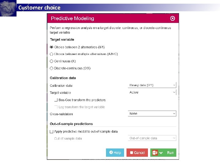
Customer choice Office Star Binary Logit Choice Example § Office Star tries to predict the likelihood that a customer will be active next quarter and make a purchase; § Data are available on the past purchase behavior of 200 customers who were classified into the active or inactive segment; § The predictor variables are gender, age, months since last purchase (recency), purchase frequency, and amount spent per purchase (average basket);

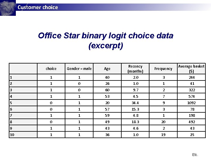
Customer choice Office Star binary logit choice data (excerpt) choice Gender = male Age 1 1 1 40 Recency (months) 2. 0 3 Average basket ($) 244 2 1 0 26 1. 0 1 41 3 1 0 60 9. 7 2 322 4 1 1 53 4. 5 7 574 5 0 1 20 34. 4 9 1092 6 0 1 57 15. 3 3 78 7 1 1 59 4. 8 1 198 8 0 1 49 18. 3 20 492 9 1 1 43 4. 6 2 43 10 1 1 36 1. 0 19 25 Frequency Etc.

Customer choice

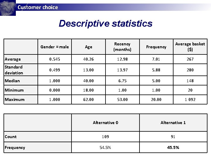
Customer choice Descriptive statistics Gender = male Age Recency (months) Frequency Average basket ($) Average 0. 545 40. 26 12. 98 7. 01 267 Standard deviation 0. 499 13. 00 13. 97 5. 88 280 Median 1. 000 40. 00 6. 75 5. 00 148 Minimum 0. 000 18. 00 1. 00 20 Maximum 1. 000 62. 00 53. 00 20. 00 1 092 Count Frequency Alternative 0 Alternative 1 109 91 54. 5% 45. 5%

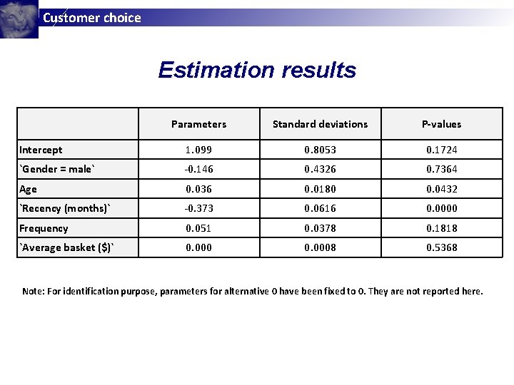
Customer choice Estimation results Parameters Standard deviations P-values Intercept 1. 099 0. 8053 0. 1724 `Gender = male` -0. 146 0. 4326 0. 7364 Age 0. 036 0. 0180 0. 0432 `Recency (months)` -0. 373 0. 0616 0. 0000 Frequency 0. 051 0. 0378 0. 1818 `Average basket ($)` 0. 0008 0. 5368 Note: For identification purpose, parameters for alternative 0 have been fixed to 0. They are not reported here.

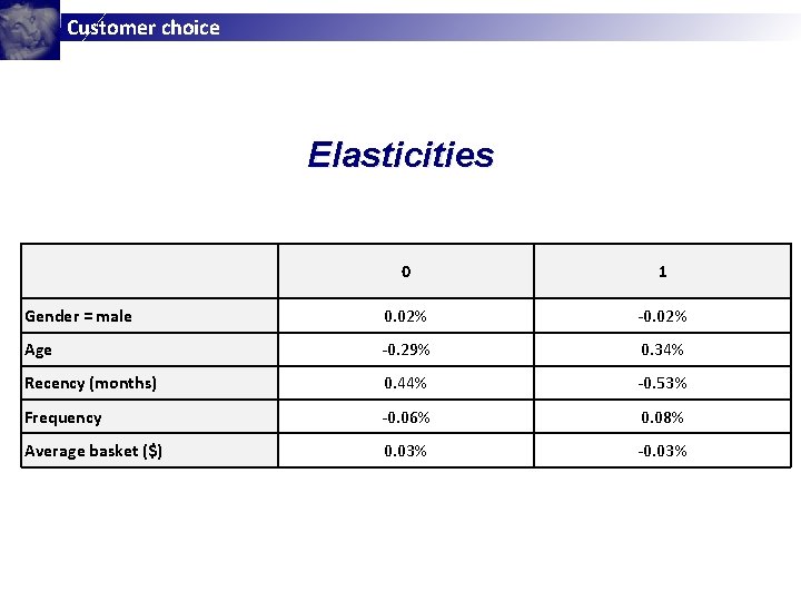
Customer choice Elasticities 0 1 Gender = male 0. 02% -0. 02% Age -0. 29% 0. 34% Recency (months) 0. 44% -0. 53% Frequency -0. 06% 0. 08% Average basket ($) 0. 03% -0. 03%

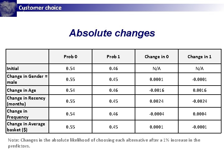
Customer choice Absolute changes Prob 0 Prob 1 Change in 0 Change in 1 Initial 0. 54 0. 46 N/A Change in Gender = male 0. 55 0. 45 0. 0001 -0. 0001 Change in Age 0. 54 0. 46 -0. 0016 0. 55 0. 45 0. 0024 -0. 0024 0. 54 0. 46 -0. 0004 0. 55 0. 45 0. 0001 -0. 0001 Change in Recency (months) Change in Frequency Change in Average basket ($) Note: Changes in the absolute likelihood of choosing each alternative after a 1% increase in the predictors.

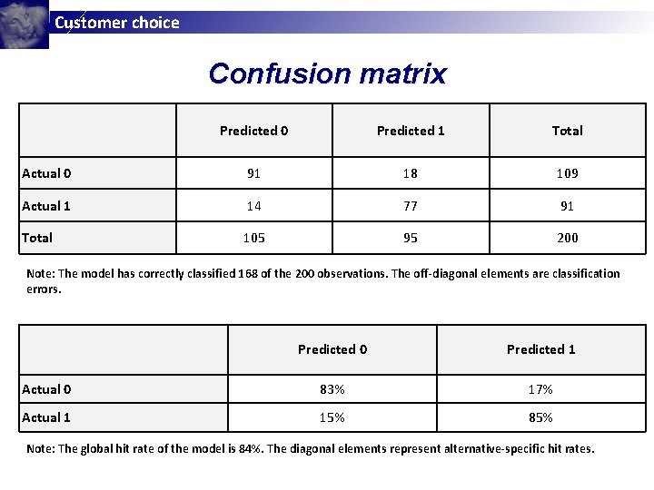
Customer choice Confusion matrix Predicted 0 Predicted 1 Total Actual 0 91 18 109 Actual 1 14 77 91 Total 105 95 200 Note: The model has correctly classified 168 of the 200 observations. The off-diagonal elements are classification errors. Predicted 0 Predicted 1 Actual 0 83% 17% Actual 1 15% 85% Note: The global hit rate of the model is 84%. The diagonal elements represent alternative-specific hit rates.

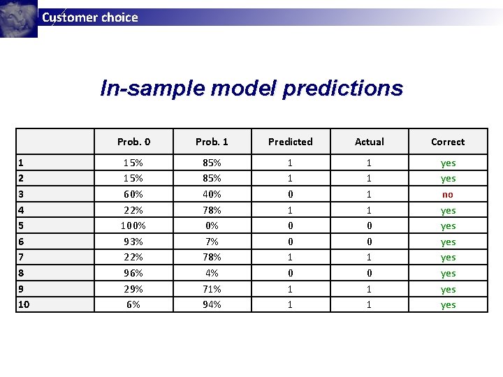
Customer choice In-sample model predictions 1 2 3 4 5 6 7 8 9 10 Prob. 1 Predicted Actual Correct 15% 60% 22% 100% 93% 22% 96% 29% 6% 85% 40% 78% 0% 7% 78% 4% 71% 94% 1 1 0 0 1 1 yes no yes yes

Customer choice Review: Basic idea of the binary choice model §

Customer choice Review: Evaluating the effect of quality on choice Model Effect of a unit (percentage) change in Q

Customer choice The generalized logit choice model

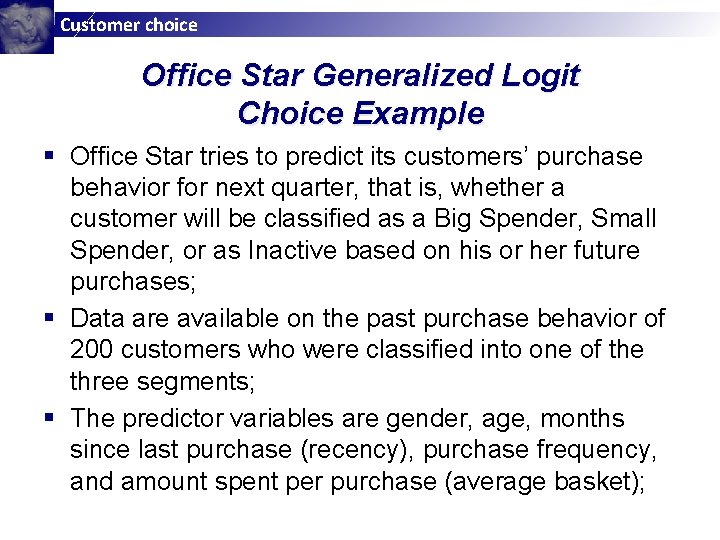
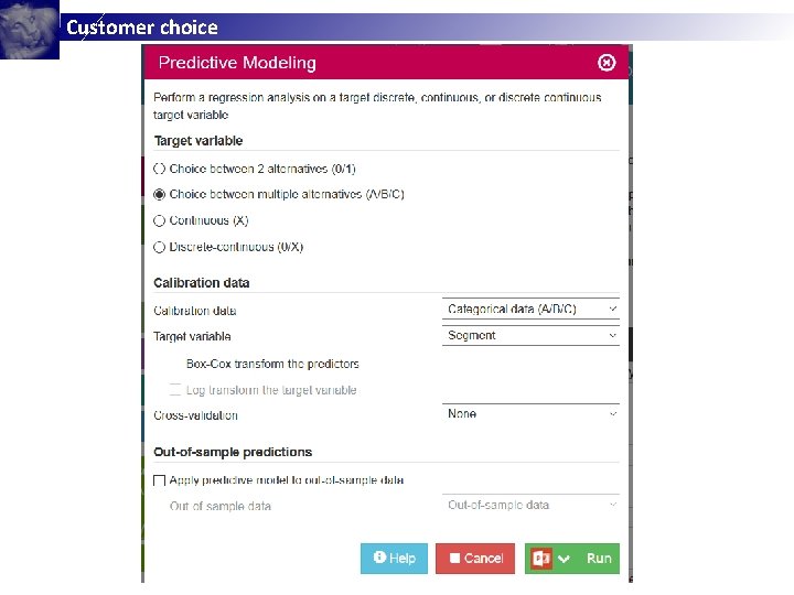
Customer choice Office Star Generalized Logit Choice Example § Office Star tries to predict its customers’ purchase behavior for next quarter, that is, whether a customer will be classified as a Big Spender, Small Spender, or as Inactive based on his or her future purchases; § Data are available on the past purchase behavior of 200 customers who were classified into one of the three segments; § The predictor variables are gender, age, months since last purchase (recency), purchase frequency, and amount spent per purchase (average basket);

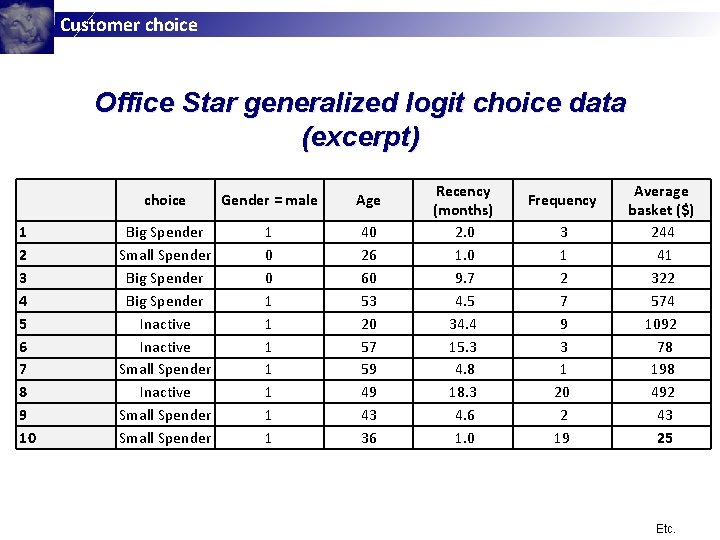
Customer choice Office Star generalized logit choice data (excerpt) 1 2 3 4 5 6 7 8 9 10 choice Gender = male Age Big Spender Small Spender Big Spender Inactive Small Spender 1 0 0 1 1 1 1 40 26 60 53 20 57 59 49 43 36 Recency (months) 2. 0 1. 0 9. 7 4. 5 34. 4 15. 3 4. 8 18. 3 4. 6 1. 0 Frequency 3 1 2 7 9 3 1 20 2 19 Average basket ($) 244 41 322 574 1092 78 198 492 43 25 Etc.

Customer choice

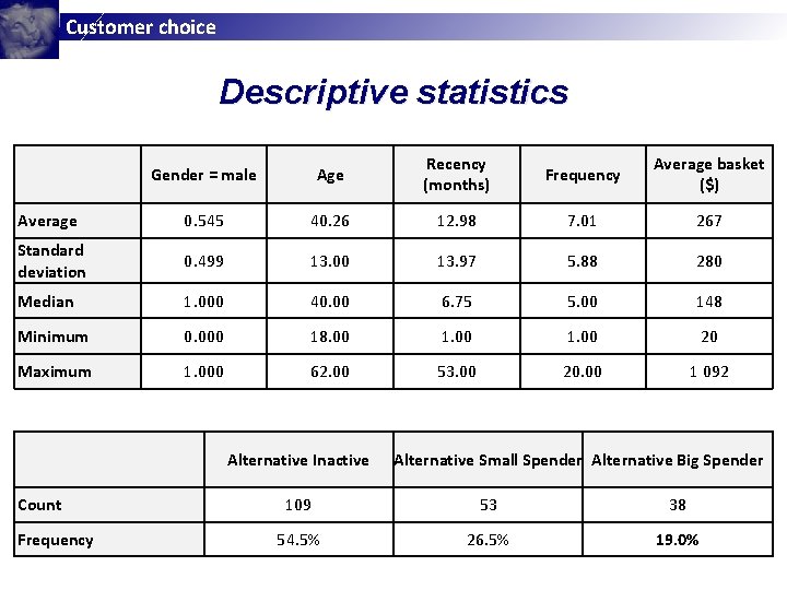
Customer choice Descriptive statistics Gender = male Age Recency (months) Frequency Average basket ($) Average 0. 545 40. 26 12. 98 7. 01 267 Standard deviation 0. 499 13. 00 13. 97 5. 88 280 Median 1. 000 40. 00 6. 75 5. 00 148 Minimum 0. 000 18. 00 1. 00 20 Maximum 1. 000 62. 00 53. 00 20. 00 1 092 Alternative Inactive Count Frequency Alternative Small Spender Alternative Big Spender 109 53 38 54. 5% 26. 5% 19. 0%

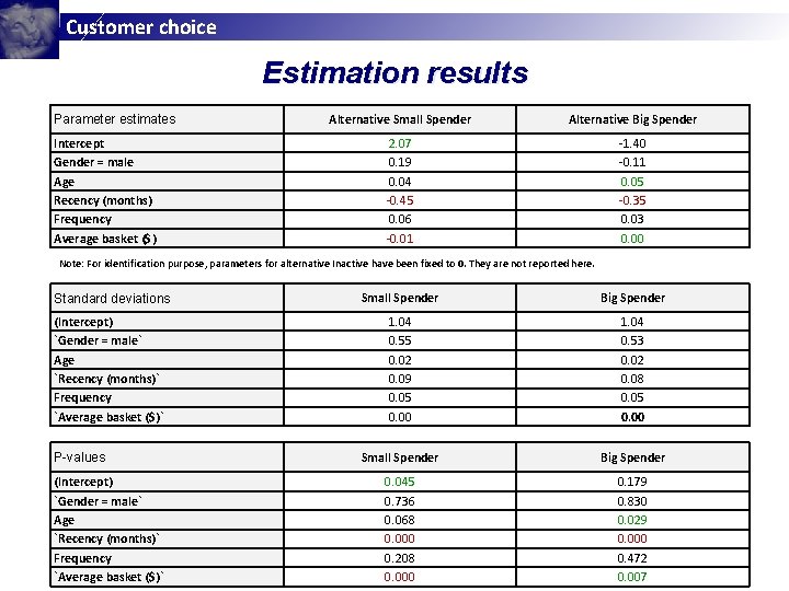
Customer choice Estimation results Parameter estimates Intercept Gender = male Age Recency (months) Frequency Average basket ($) Alternative Small Spender Alternative Big Spender 2. 07 0. 19 0. 04 -0. 45 0. 06 -0. 01 -1. 40 -0. 11 0. 05 -0. 35 0. 03 0. 00 Note: For identification purpose, parameters for alternative Inactive have been fixed to 0. They are not reported here. Standard deviations Small Spender Big Spender (Intercept) `Gender = male` Age `Recency (months)` Frequency `Average basket ($)` 1. 04 0. 55 0. 02 0. 09 0. 05 0. 00 1. 04 0. 53 0. 02 0. 08 0. 05 0. 00 Small Spender Big Spender 0. 045 0. 736 0. 068 0. 000 0. 208 0. 000 0. 179 0. 830 0. 029 0. 000 0. 472 0. 007 P-values (Intercept) `Gender = male` Age `Recency (months)` Frequency `Average basket ($)`

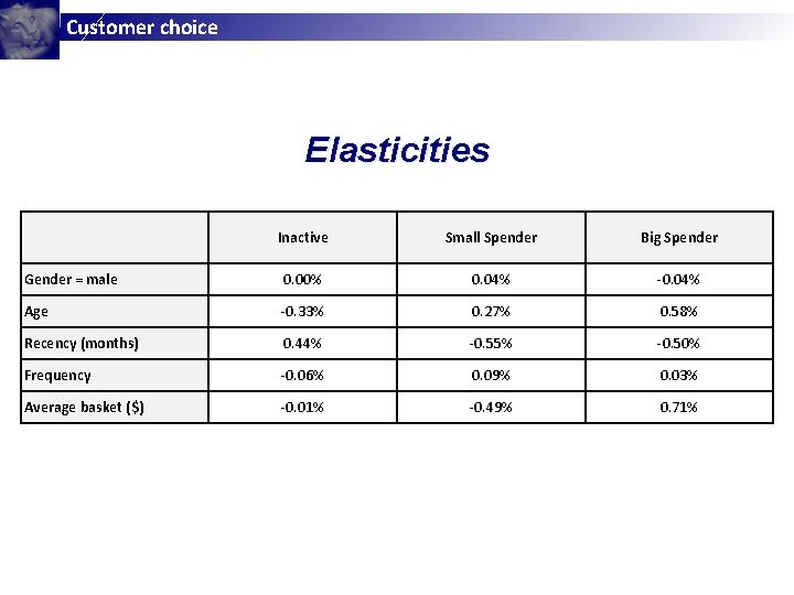
Customer choice Elasticities Inactive Small Spender Big Spender Gender = male 0. 00% 0. 04% -0. 04% Age -0. 33% 0. 27% 0. 58% Recency (months) 0. 44% -0. 55% -0. 50% Frequency -0. 06% 0. 09% 0. 03% Average basket ($) -0. 01% -0. 49% 0. 71%

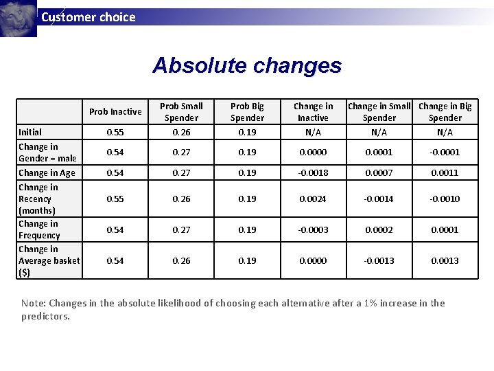
Customer choice Absolute changes Prob Inactive Prob Small Spender Prob Big Spender Change in Inactive Initial 0. 55 0. 26 0. 19 N/A N/A Change in Gender = male 0. 54 0. 27 0. 19 0. 0000 0. 0001 -0. 0001 Change in Age 0. 54 0. 27 0. 19 -0. 0018 0. 0007 0. 0011 0. 55 0. 26 0. 19 0. 0024 -0. 0010 0. 54 0. 27 0. 19 -0. 0003 0. 0002 0. 0001 0. 54 0. 26 0. 19 0. 0000 -0. 0013 Change in Recency (months) Change in Frequency Change in Average basket ($) Change in Small Change in Big Spender Note: Changes in the absolute likelihood of choosing each alternative after a 1% increase in the predictors.

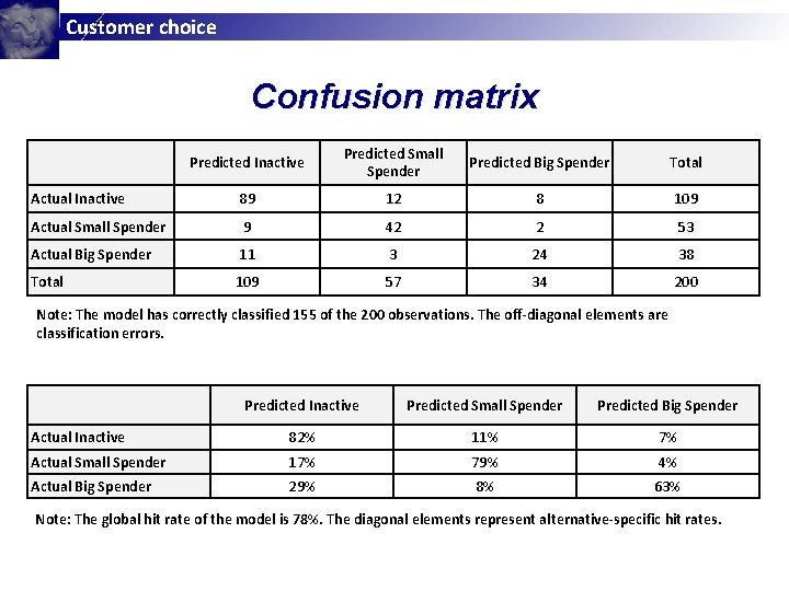
Customer choice Confusion matrix Predicted Inactive Predicted Small Spender Predicted Big Spender Total Actual Inactive 89 12 8 109 Actual Small Spender 9 42 2 53 Actual Big Spender 11 3 24 38 Total 109 57 34 200 Note: The model has correctly classified 155 of the 200 observations. The off-diagonal elements are classification errors. Predicted Inactive Predicted Small Spender Predicted Big Spender Actual Inactive 82% 11% 7% Actual Small Spender 17% 79% 4% Actual Big Spender 29% 8% 63% Note: The global hit rate of the model is 78%. The diagonal elements represent alternative-specific hit rates.

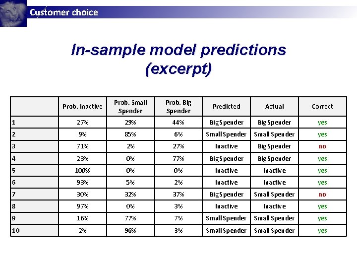
Customer choice In-sample model predictions (excerpt) Prob. Inactive Prob. Small Spender Prob. Big Spender Predicted Actual Correct 1 27% 29% 44% Big Spender yes 2 9% 85% 6% Small Spender yes 3 71% 2% 27% Inactive Big Spender no 4 23% 0% 77% Big Spender yes 5 100% 0% 0% Inactive yes 6 93% 5% 2% Inactive yes 7 30% 32% 37% Big Spender Small Spender no 8 97% 0% 3% Inactive yes 9 16% 77% 7% Small Spender yes 10 2% 96% 3% Small Spender yes

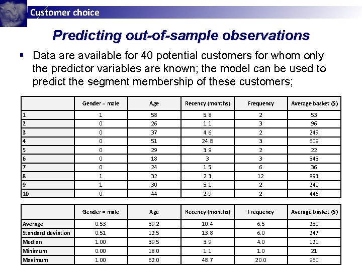
Customer choice Predicting out-of-sample observations § Data are available for 40 potential customers for whom only the predictor variables are known; the model can be used to predict the segment membership of these customers; Gender = male Age Recency (months) Frequency Average basket ($) 1 0 0 0 1 1 0 58 26 37 51 29 18 24 32 30 44 5. 8 1. 1 4. 6 24. 8 3. 9 3 1. 5 2. 3 5. 1 2. 9 2 3 2 3 6 12 2 2 53 96 249 609 22 545 36 893 240 446 Gender = male Age Recency (months) Frequency Average basket ($) Average 0. 53 39. 2 10. 4 6. 5 230 Standard deviation 0. 51 12. 5 13. 8 6. 0 247 Median 1. 00 39. 5 3. 9 4. 0 121 Minimum 0. 00 18. 0 1. 1 1. 0 21 Maximum 1. 00 62. 0 48. 7 20. 0 960 1 2 3 4 5 6 7 8 9 10

Customer choice Frequency table for predicted choices Count Frequency Alternative Inactive Alternative Small Spender Alternative Big Spender 18. 0 15. 0 7. 0 45. 0% 37. 5% 17. 5%

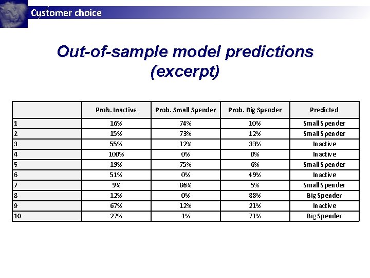
Customer choice Out-of-sample model predictions (excerpt) 1 2 3 4 5 6 7 8 9 10 Prob. Inactive Prob. Small Spender Prob. Big Spender Predicted 16% 15% 55% 100% 19% 51% 9% 12% 67% 27% 74% 73% 12% 0% 75% 0% 86% 0% 12% 1% 10% 12% 33% 0% 6% 49% 5% 88% 21% 71% Small Spender Inactive Small Spender Big Spender Inactive Big Spender

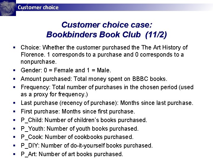
Customer choice case: Bookbinders Book Club (11/2) § Choice: Whether the customer purchased the The Art History of Florence. 1 corresponds to a purchase and 0 corresponds to a nonpurchase. § Gender: 0 = Female and 1 = Male. § Amount purchased: Total money spent on BBBC books. § Frequency: Total number of purchases in the chosen period (used as a proxy for frequency. ) § Last purchase (recency of purchase): Months since last purchase. § First purchase: Months since first purchase. § P_Child: Number of children’s books purchased. § P_Youth: Number of youth books purchased. § P_Cook: Number of cookbooks purchased. § P_DIY: Number of do-it-yourself books purchased. § P_Art: Number of art books purchased.

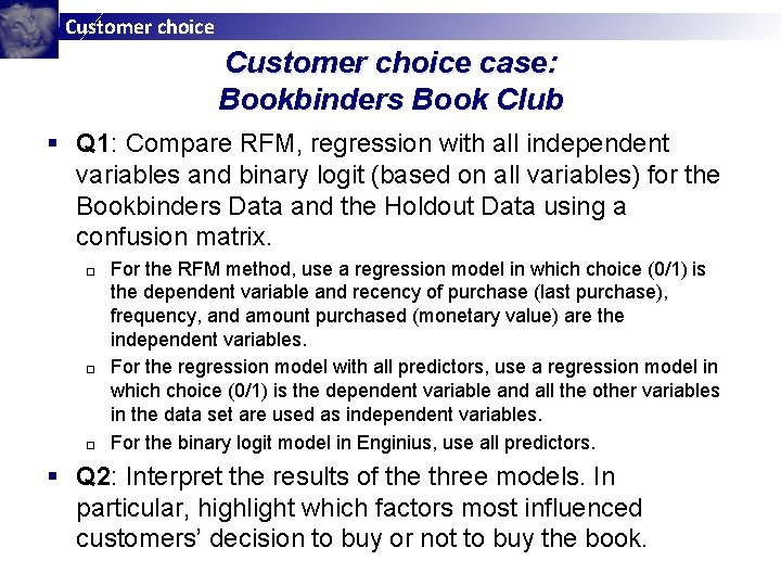
Customer choice case: Bookbinders Book Club § Q 1: Compare RFM, regression with all independent variables and binary logit (based on all variables) for the Bookbinders Data and the Holdout Data using a confusion matrix. For the RFM method, use a regression model in which choice (0/1) is the dependent variable and recency of purchase (last purchase), frequency, and amount purchased (monetary value) are the independent variables. □ For the regression model with all predictors, use a regression model in which choice (0/1) is the dependent variable and all the other variables in the data set are used as independent variables. □ For the binary logit model in Enginius, use all predictors. □ § Q 2: Interpret the results of the three models. In particular, highlight which factors most influenced customers’ decision to buy or not to buy the book.

Customer choice case: Bookbinders Book Club § RFM model: Predicted P[Choice] = a + b 1*R + b 2*F + b 3*M § If P[Choice] <. 5, predicted choice = 0, else predicted choice = 1; § Cross-classify predicted choices with actual choices;

Customer choice Assignments for next three classes § Wednesday 10/20 □ Wrap up customer choice § Monday 10/25 □ Northern Aero CLV case § Wednesday 10/27 Download the overheads (conjoint. pptx or conjoint. pdf) □ Read LRB Chapter 6 (esp. pp. 178 -190) □ Read Conjoint Analysis Tutorial (Enginius) □