Curve Fitting Splines 1 Why Spline Interpolation To

Curve Fitting: Splines 1

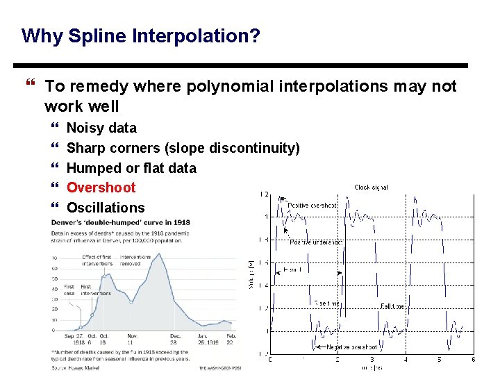
Why Spline Interpolation? } To remedy where polynomial interpolations may not work well } } } Noisy data Sharp corners (slope discontinuity) Humped or flat data Overshoot Oscillations

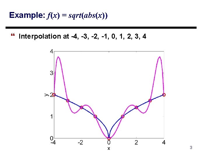
Example: f(x) = sqrt(abs(x)) } Interpolation at -4, -3, -2, -1, 0, 1, 2, 3, 4 3

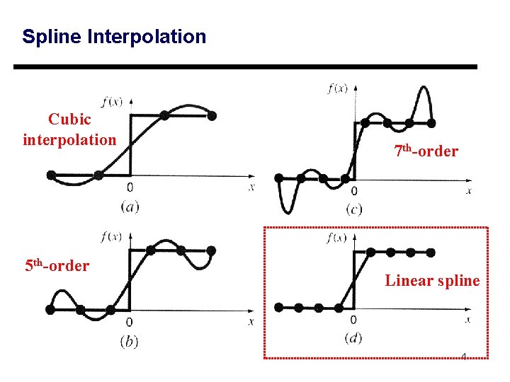
Spline Interpolation Cubic interpolation 5 th-order 7 th-order Linear spline 4

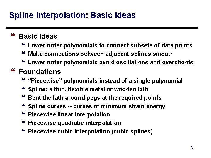
Spline Interpolation: Basic Ideas } Lower order polynomials to connect subsets of data points } Make connections between adjacent splines smooth } Lower order polynomials avoid oscillations and overshoots } Foundations } } } } “Piecewise” polynomials instead of a single polynomial Spline: a thin, flexible metal or wooden lath Bent the lath around pegs at the required points Spline curves -- curves of minimum strain energy Piecewise linear interpolation Piecewise quadratic interpolation Piecewise cubic interpolation (cubic splines) 5

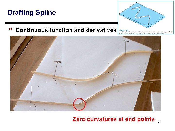
Drafting Spline } Continuous function and derivatives Zero curvatures at end points 6

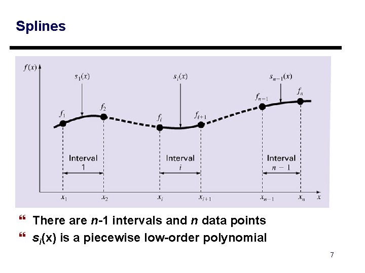
Splines } There are n-1 intervals and n data points } si(x) is a piecewise low-order polynomial 7

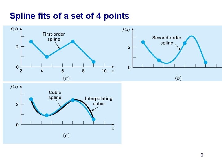
Spline fits of a set of 4 points 8

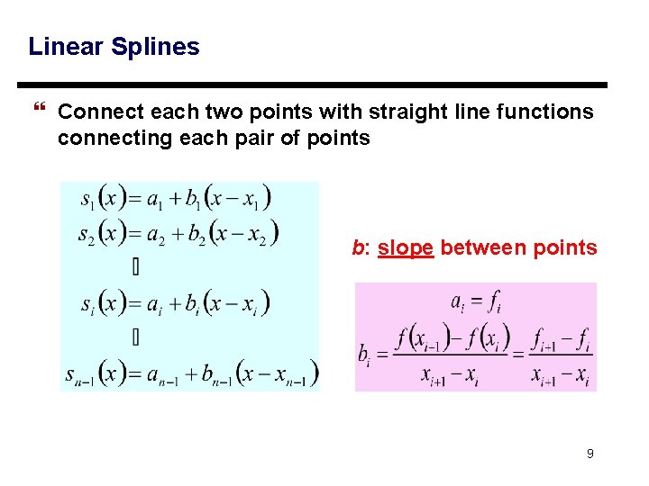
Linear Splines } Connect each two points with straight line functions connecting each pair of points b: slope between points 9

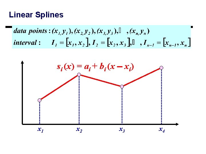
Linear Splines si (x) = ai + bi (x xi) x 1 x 2 x 3 x 4

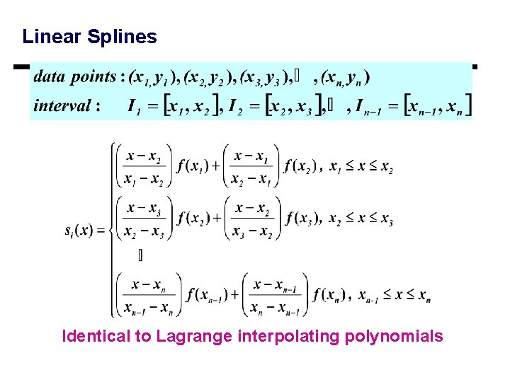
Linear Splines Identical to Lagrange interpolating polynomials

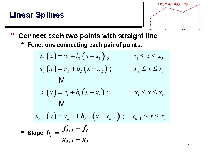
Linear Splines } Connect each two points with straight line } Functions connecting each pair of points: } Slope 12

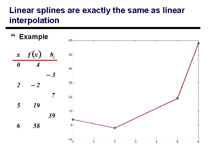
Linear splines are exactly the same as linear interpolation } Example 13

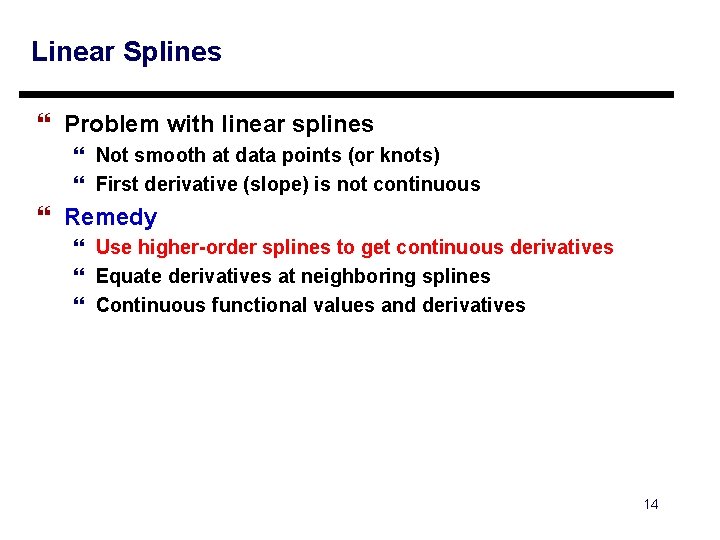
Linear Splines } Problem with linear splines } Not smooth at data points (or knots) } First derivative (slope) is not continuous } Remedy } Use higher-order splines to get continuous derivatives } Equate derivatives at neighboring splines } Continuous functional values and derivatives 14

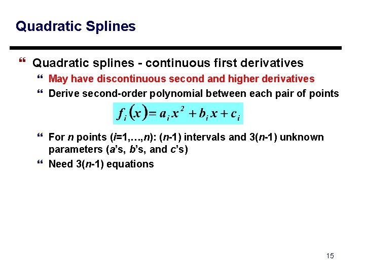
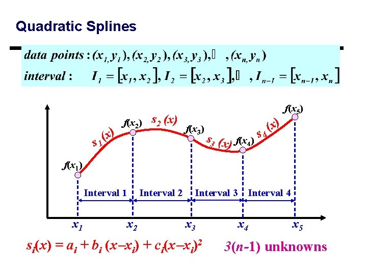
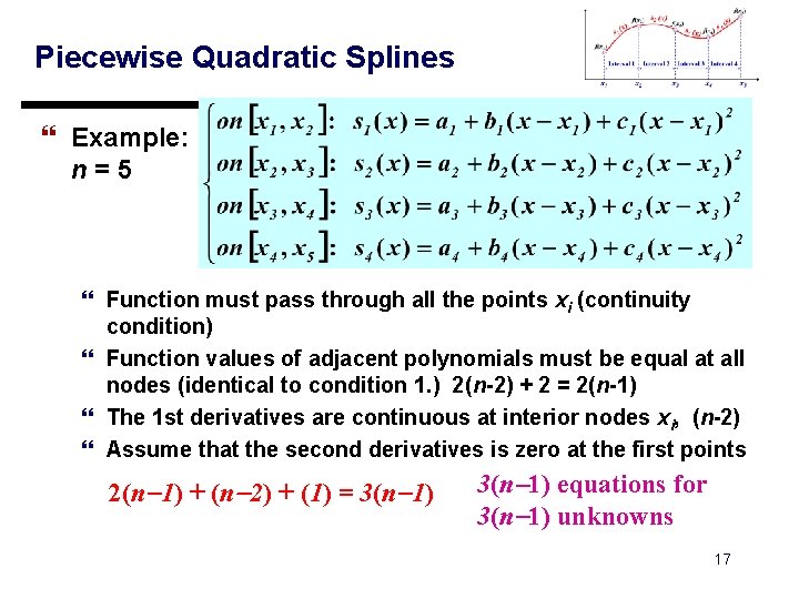
Quadratic Splines } Quadratic splines - continuous first derivatives } May have discontinuous second and higher derivatives } Derive second-order polynomial between each pair of points } For n points (i=1, …, n): (n-1) intervals and 3(n-1) unknown parameters (a’s, b’s, and c’s) } Need 3(n-1) equations 15

Quadratic Splines x) ( s 1 f(x 2) s 2 (x) f(x 3) s 3 (x) f(x 4) s 4 (x) f(x 5) f(x 1) Interval 1 x 2 Interval 3 x 3 si(x) = ai + bi (x xi) + ci(x xi)2 Interval 4 x 5 3(n-1) unknowns

Piecewise Quadratic Splines } Example: n=5 } Function must pass through all the points xi (continuity condition) } Function values of adjacent polynomials must be equal at all nodes (identical to condition 1. ) 2(n-2) + 2 = 2(n-1) } The 1 st derivatives are continuous at interior nodes xi, (n-2) } Assume that the second derivatives is zero at the first points 2(n 1) + (n 2) + (1) = 3(n 1) equations for 3(n 1) unknowns 17

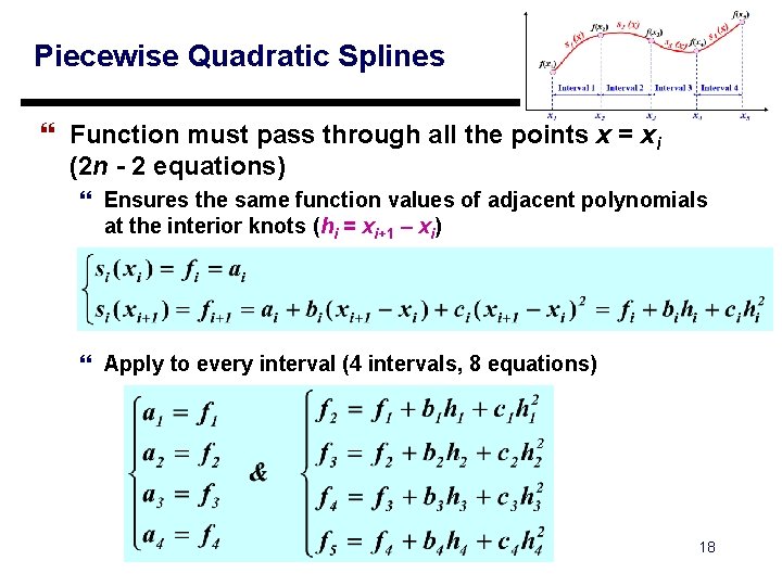
Piecewise Quadratic Splines } Function must pass through all the points x = xi (2 n - 2 equations) } Ensures the same function values of adjacent polynomials at the interior knots (hi = xi+1 – xi) } Apply to every interval (4 intervals, 8 equations) 18

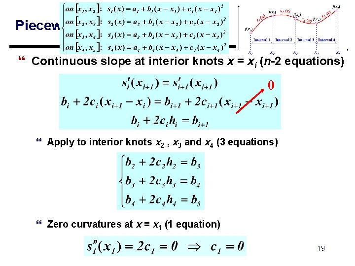
Piecewise Quadratic Splines } Continuous slope at interior knots x = xi (n-2 equations) 0 } Apply to interior knots x 2 , x 3 and x 4 (3 equations) } Zero curvatures at x = x 1 (1 equation) 19

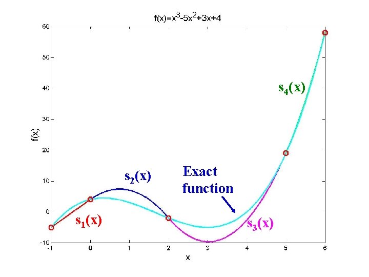
Example: Quadratic Spline

Quadratic Spline Interpolation function [A, b] = quadratic(x, f) % exact solution f(x)=x^3 -5 x^2+3 x+4 % x=[-1 0 2 5 6]; f=[-5 4 -2 19 58]; h 1=x(2)-x(1); h 2=x(3)-x(2); h 3=x(4)-x(3); h 4=x(5)-x(4); f 1=f(1); f 2=f(2); f 3=f(3); f 4=f(4); f 5=f(5); A=[1 0 0 0 h 1^2 0 0 0 1 0 0 0 h 2^2 0 0 0 1 0 0 0 h 3^2 0 0 0 1 0 0 0 h 4^2 0 1 2*h 1 0 -1 0 0 0 1 2*h 2 0 -1 0 0 0 1 2*h 3 0 -1 0 0 0 0]; 21 b=[f 1; f 2 -f 1; f 2; f 3 -f 2; f 3; f 4 -f 3; f 4; f 5 -f 4; 0; 0];

>> x=[-1 0 2 5 6]; f=[-5 4 -2 19 58]; >> [A, b]=quadratic(x, f) p = Ab -5. 0000 9. 0000 0 4. 0000 9. 0000 -6. 0000 -2. 0000 -15. 0000 7. 3333 19. 0000 29. 0000 10. 0000 dx = 0. 1; z 1=x(1): dx: x(2); s 1=p(1)+p(2)*(z 1 -x(1))+p(3)*(z 1 -x(1)). ^2; z 2=x(2): dx: x(3); s 2=p(4)+p(5)*(z 2 -x(2))+p(6)*(z 2 -x(2)). ^2; z 3=x(3): dx: x(4); s 3=p(7)+p(8)*(z 3 -x(3))+p(9)*(z 3 -x(3)). ^2; z 4=x(4): dx: x(5); s 4=p(10)+p(11)*(z 4 -x(4))+p(12)*(z 4 -x(4)). ^2; H=plot(z 1, s 1, 'r', z 2, s 2, 'b', z 3, s 3, 'm', z 4, s 4, 'g'); xx=-1: 0. 1: 6; fexact=xx. ^3 -5*xx. ^2+3*xx+4; hold on; G=plot(xx, fexact, 'c', x, f, 'ro'); set(H, 'Line. Width', 3); set(G, 'Line. Width', 3, 'Marker. Size', 8); H 1=xlabel('x'); set(H 1, 'Font. Size', 15); H 2=ylabel('f(x)'); set(H 2, 'Font. Size', 15); H 3=title('f(x)=x^3 -5 x^2+3 x+4'); set(H 3, 'Font. Size', 15);

s 4(x) s 2(x) s 1(x) Exact function s 3(x)

Practice: Re-visit the US population problem at the end of Unit 13 and see how the spline method works

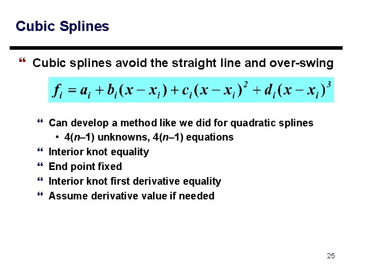
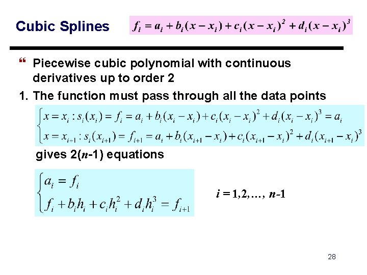
Cubic Splines } Cubic splines avoid the straight line and over-swing } Can develop a method like we did for quadratic splines • 4(n– 1) unknowns, 4(n– 1) equations } Interior knot equality } End point fixed } Interior knot first derivative equality } Assume derivative value if needed 25

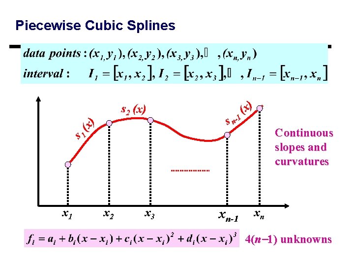
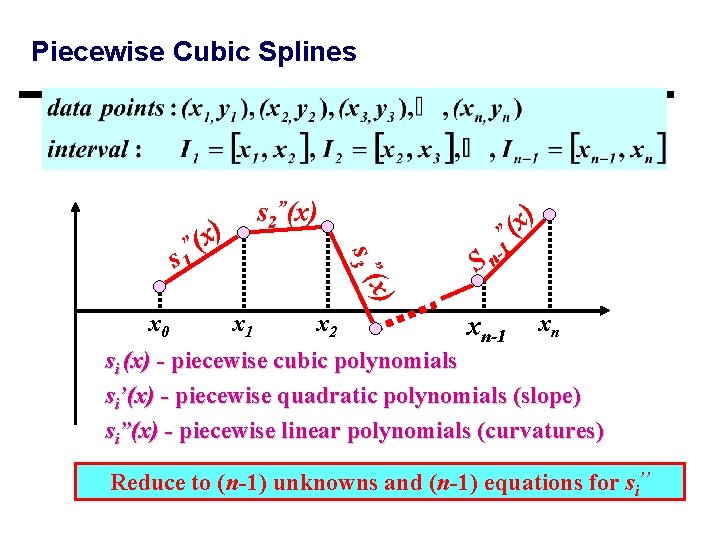
Piecewise Cubic Splines s n-1 (x) Continuous slopes and curvatures s 1 (x ) s 2 (x) x 1 x 2 x 3 xn-1 xn 4(n 1) unknowns

Piecewise Cubic Splines s 2”(x) ) ” s 3 ( ” (x s 1 ) x ”( 1 n S x) x 0 x 1 x 2 xn-1 xn si (x) - piecewise cubic polynomials si’(x) - piecewise quadratic polynomials (slope) si”(x) - piecewise linear polynomials (curvatures) Reduce to (n-1) unknowns and (n-1) equations for si’’

Cubic Splines } Piecewise cubic polynomial with continuous derivatives up to order 2 1. The function must pass through all the data points gives 2(n-1) equations i = 1, 2, …, n-1 28

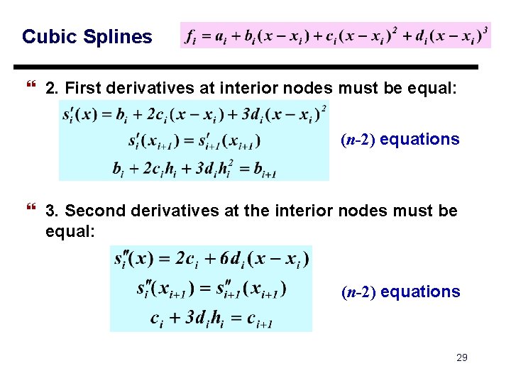
Cubic Splines } 2. First derivatives at interior nodes must be equal: (n-2) equations } 3. Second derivatives at the interior nodes must be equal: (n-2) equations 29

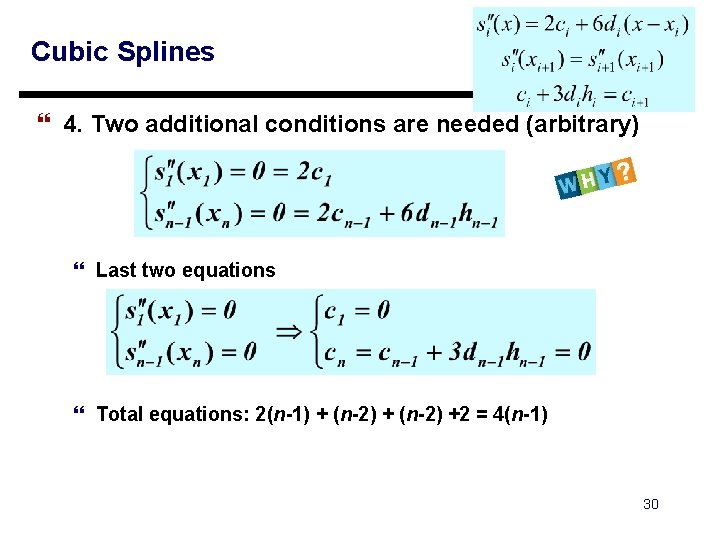
Cubic Splines } 4. Two additional conditions are needed (arbitrary) } Last two equations } Total equations: 2(n-1) + (n-2) +2 = 4(n-1) 30

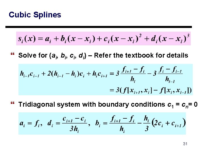
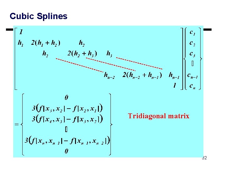
Cubic Splines } Solve for (ai, bi, ci, di) – Refer the textbook for details } Tridiagonal system with boundary conditions c 1 = cn= 0 31

Cubic Splines Tridiagonal matrix 32

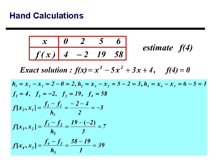
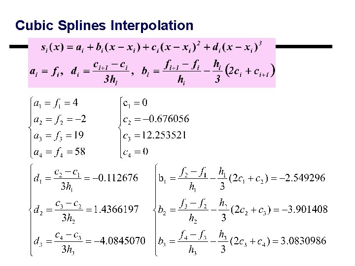
Hand Calculations 33

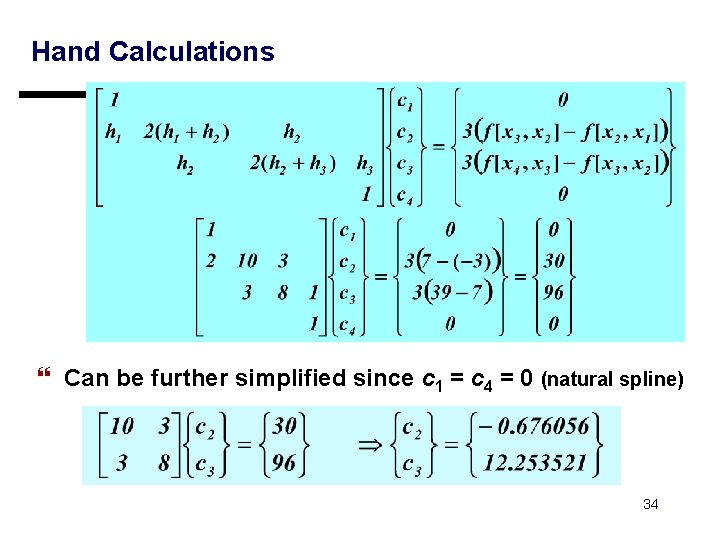
Hand Calculations } Can be further simplified since c 1 = c 4 = 0 (natural spline) 34

Cubic Splines Interpolation

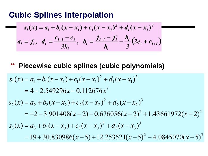
Cubic Splines Interpolation } Piecewise cubic splines (cubic polynomials)

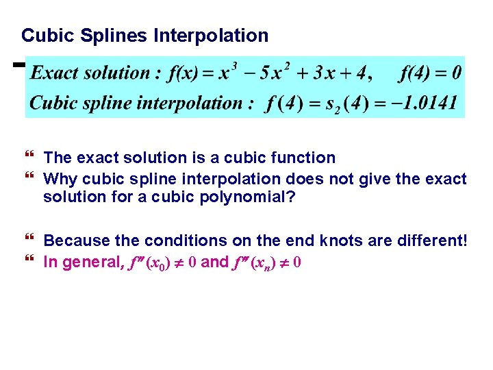
Cubic Splines Interpolation } The exact solution is a cubic function } Why cubic spline interpolation does not give the exact solution for a cubic polynomial? } Because the conditions on the end knots are different! } In general, f (x 0) 0 and f (xn) 0

So, program? Try to finish the program

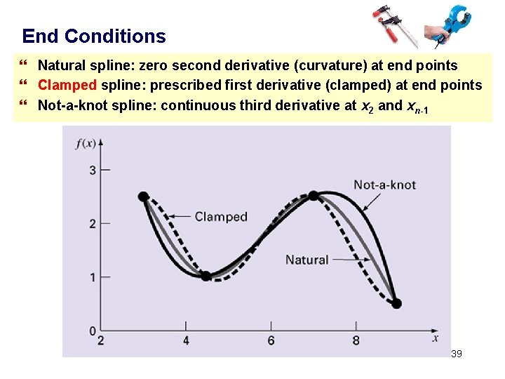
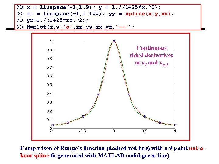
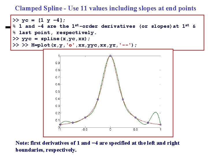
End Conditions } Natural spline: zero second derivative (curvature) at end points } Clamped spline: prescribed first derivative (clamped) at end points } Not-a-knot spline: continuous third derivative at x 2 and xn-1 39

>> >> x = linspace(-1, 1, 9); y = 1. /(1+25*x. ^2); xx = linspace(-1, 1, 100); yy = spline(x, y, xx); yr=1. /(1+25*xx. ^2); H=plot(x, y, 'o', xx, yy, xx, yr, '--'); Continuous third derivatives at x 2 and xn-1 Comparison of Runge’s function (dashed red line) with a 9 -point not-aknot spline fit generated with MATLAB (solid green line)

Clamped Spline - Use 11 values including slopes at end points >> yc = [1 y – 4]; % 1 and -4 are the 1 st-order derivatives (or slopes)at 1 st & % last point, respectively. >> yyc = spline(x, yc, xx); >> >> H=plot(x, y, 'o', xx, yyc, xx, yr, '--'); Note: first derivatives of 1 and 4 are specified at the left and right boundaries, respectively.

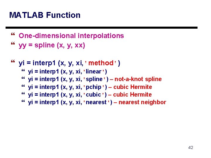
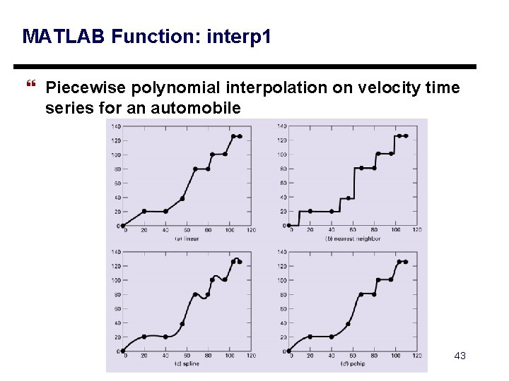
MATLAB Function } One-dimensional interpolations } yy = spline (x, y, xx) } yi = interp 1 (x, y, xi, 'method') } } } yi = interp 1 (x, y, xi, 'linear') yi = interp 1 (x, y, xi, 'spline') – not-a-knot spline yi = interp 1 (x, y, xi, 'pchip') – cubic Hermite yi = interp 1 (x, y, xi, 'cubic') – cubic Hermite yi = interp 1 (x, y, xi, 'nearest') – nearest neighbor 42

MATLAB Function: interp 1 } Piecewise polynomial interpolation on velocity time series for an automobile 43

MATLAB Function: interp 1 >> x=[1 2 4 7 9 10] x = 1 2 4 7 9 10 4 9 2 >> y=[3 -2 5 4 9 2] y = 3 -2 5 >> xi=1: 0. 1: 10; >> y 1=interp 1(x, y, xi, 'linear'); >> y 2=interp 1(x, y, xi, 'spline'); >> y 3=interp 1(x, y, xi, 'cubic'); >> plot(x, y, 'ro', xi, y 1, xi, y 2, xi, y 3, 'Line. Width', 2, 'Marker. Size', 12) >> print -djpeg spline 00. jpg 44

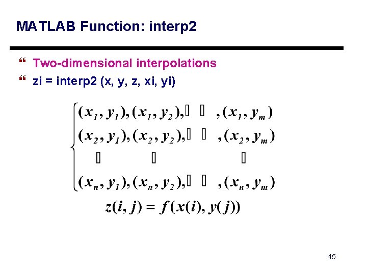
MATLAB Function: interp 2 } Two-dimensional interpolations } zi = interp 2 (x, y, z, xi, yi) 45

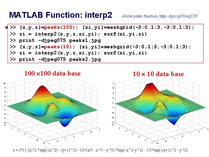
MATLAB Function: interp 2 >> >> >> About peaks function, https: //goo. gl/9 sm. QCN [x, y, z]=peaks(100); [xi, yi]=meshgrid(-3: 0. 1: 3, -3: 0. 1: 3); zi = interp 2(x, y, z, xi, yi); surf(xi, yi, zi) print -djpeg 075 peaks 1. jpg [x, y, z]=peaks(10); [xi, yi]=meshgrid(-3: 0. 1: 3, -3: 0. 1: 3); zi = interp 2(x, y, z, xi, yi); surf(xi, yi, zi) print -djpeg 075 peaks 2. jpg 100 data base 10 data base z = 3*(1 -x). ^2. *exp(-(x. ^2) - (y+1). ^2) - 10*(x/5 - x. ^3 - y. ^5). *exp(-x. ^2 -y. ^2) - 1/3*exp(-(x+1). ^2 - y. ^2)