CTF Analysis and Terminal Loss P UCC Time

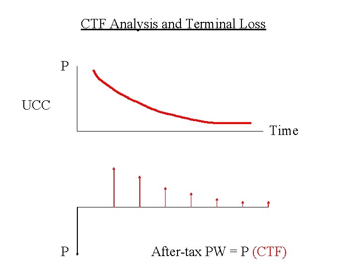
CTF Analysis and Terminal Loss P UCC Time P After-tax PW = P (CTF)

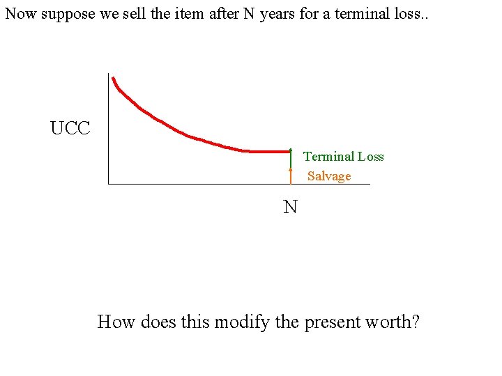
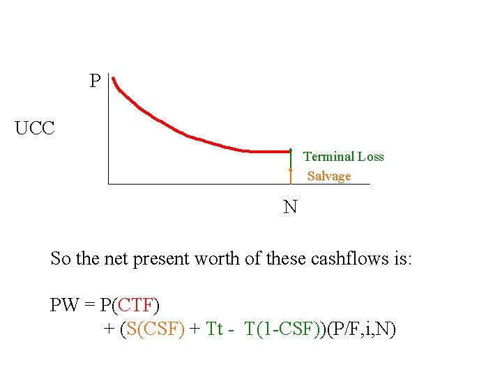
Now suppose we sell the item after N years for a terminal loss. . UCC Terminal Loss Salvage N How does this modify the present worth?

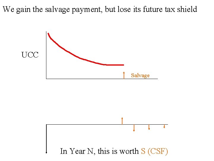
We gain the salvage payment, but lose its future tax shield UCC Salvage In Year N, this is worth S (CSF)

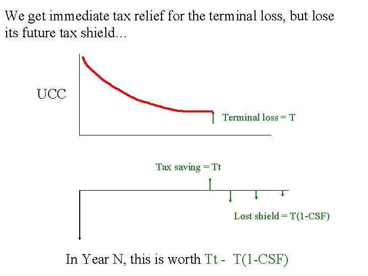
We get immediate tax relief for the terminal loss, but lose its future tax shield… UCC Terminal loss = T Tax saving = Tt Lost shield = T(1 -CSF) In Year N, this is worth Tt - T(1 -CSF)

P UCC Terminal Loss Salvage N So the net present worth of these cashflows is: PW = P(CTF) + (S(CSF) + Tt - T(1 -CSF))(P/F, i, N)

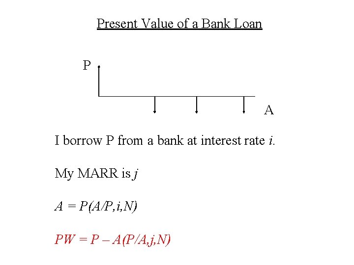
Present Value of a Bank Loan P A I borrow P from a bank at interest rate i. My MARR is j A = P(A/P, i, N) PW = P – A(P/A, j, N)

Uncertainty Analysis November 10, 2014

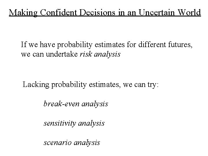
Making Confident Decisions in an Uncertain World If we have probability estimates for different futures, we can undertake risk analysis Lacking probability estimates, we can try: break-even analysis sensitivity analysis scenario analysis

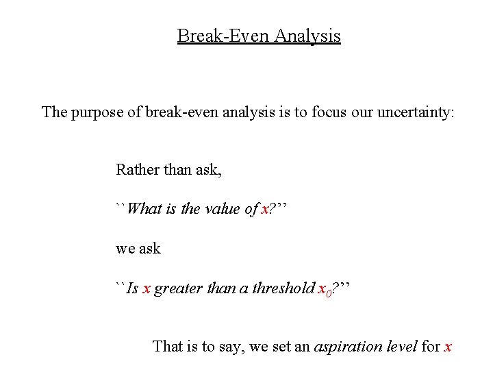
Break-Even Analysis The purpose of break-even analysis is to focus our uncertainty: Rather than ask, ``What is the value of x? ’’ we ask ``Is x greater than a threshold x 0? ’’ That is to say, we set an aspiration level for x

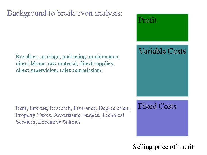
Background to break-even analysis: Royalties, spoilage, packaging, maintenance, direct labour, raw material, direct supplies, direct supervision, sales commissions Rent, Interest, Research, Insurance, Depreciation, Property Taxes, Advertising Budget, Technical Services, Executive Salaries Profit Variable Costs Fixed Costs Selling price of 1 unit

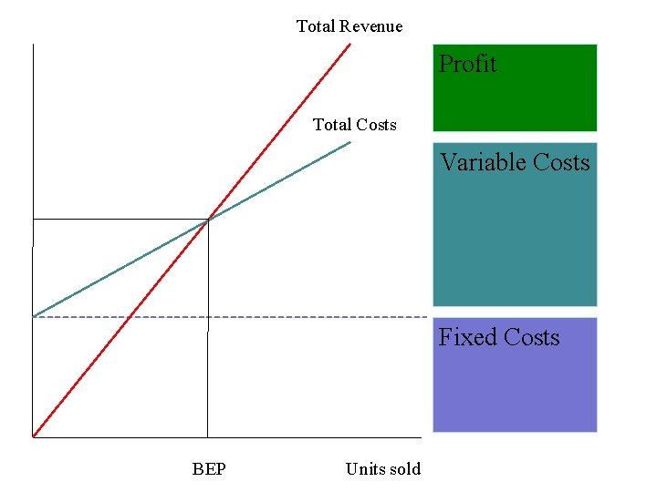
Total Revenue Profit Total Costs Variable Costs Fixed Costs BEP Units sold

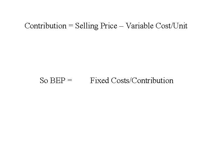
Contribution = Selling Price – Variable Cost/Unit So BEP = Fixed Costs/Contribution

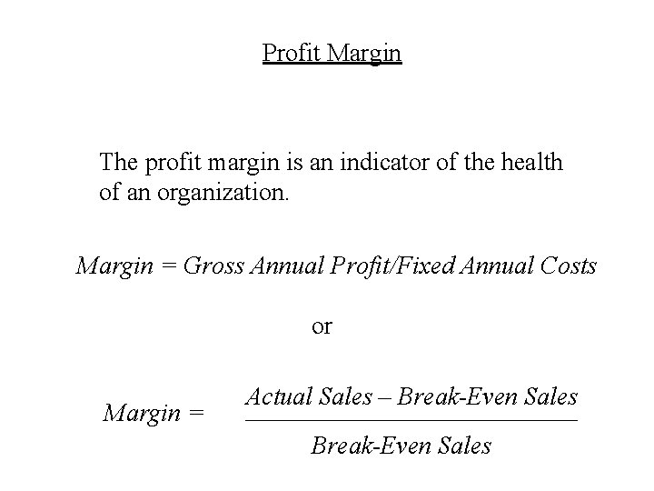
Profit Margin The profit margin is an indicator of the health of an organization. Margin = Gross Annual Profit/Fixed Annual Costs or Margin = Actual Sales – Break-Even Sales

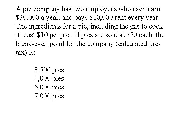
A pie company has two employees who each earn $30, 000 a year, and pays $10, 000 rent every year. The ingredients for a pie, including the gas to cook it, cost $10 per pie. If pies are sold at $20 each, the break-even point for the company (calculated pretax) is: 3, 500 pies 4, 000 pies 6, 000 pies 7, 000 pies

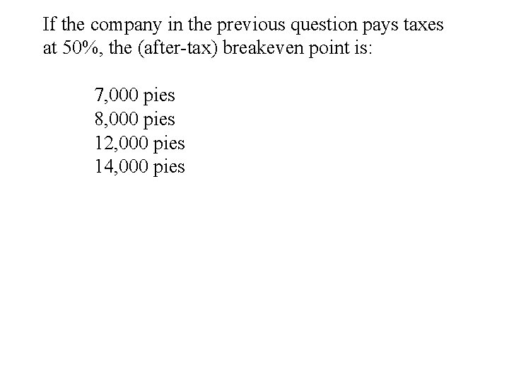
If the company in the previous question pays taxes at 50%, the (after-tax) breakeven point is: 7, 000 pies 8, 000 pies 12, 000 pies 14, 000 pies

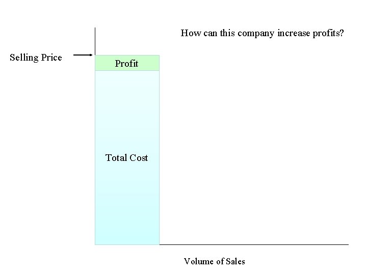
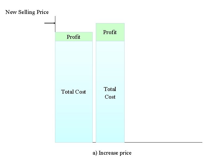
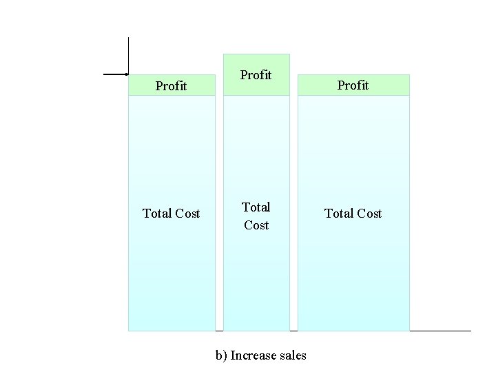
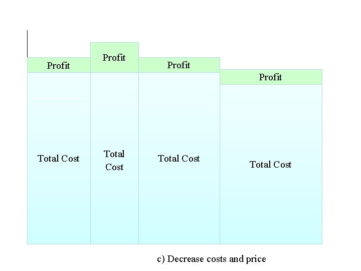
How can this company increase profits? Selling Price Profit Total Cost Volume of Sales

New Selling Price Profit Total Cost a) Increase price

Profit Total Cost b) Increase sales Profit Total Cost

Profit Total Cost c) Decrease costs and price

Example: A firm makes units that sell for $35, 000 each. Variable costs are $20, 000/unit and fixed costs are $600, 000. The plant can produce 80 units a year, but is currently only working at 60% capacity. The firm is considering reducing selling price by $2, 000/unit, adding a feature to each unit that increases variable costs by $1, 000, and spending $120, 000 on ads to increase sales. If these measures increase sales to 72 units per year, what happens to the BEP and the profit margin? Suppose instead the firm went to 200% capacity and sold the extra units at $25 K each, how would this affect gross profits?

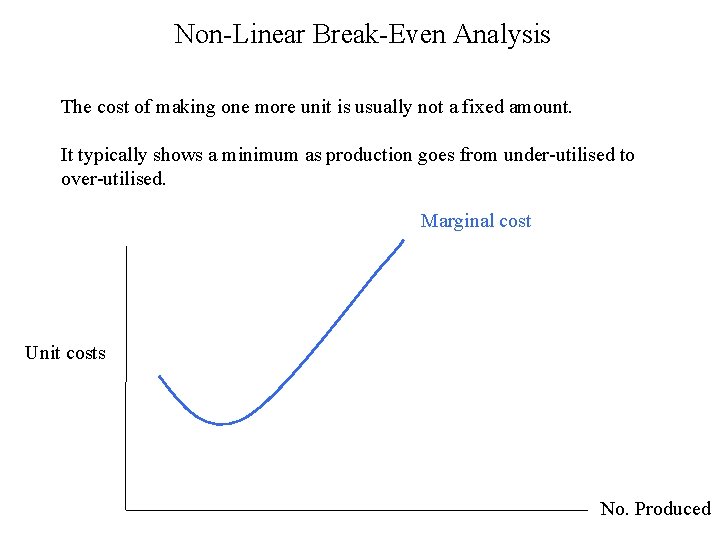
Non-Linear Break-Even Analysis The cost of making one more unit is usually not a fixed amount. It typically shows a minimum as production goes from under-utilised to over-utilised. Marginal cost Unit costs No. Produced

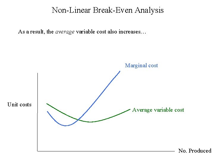
Non-Linear Break-Even Analysis As a result, the average variable cost also increases… Marginal cost Unit costs Average variable cost No. Produced

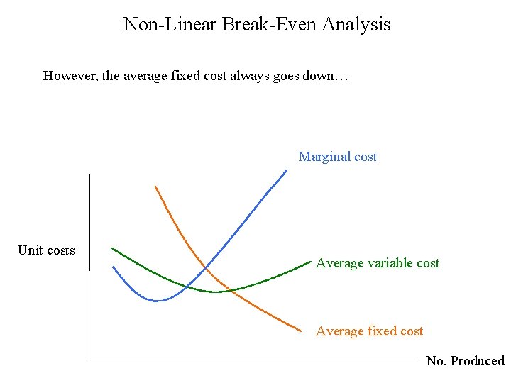
Non-Linear Break-Even Analysis However, the average fixed cost always goes down… Marginal cost Unit costs Average variable cost Average fixed cost No. Produced

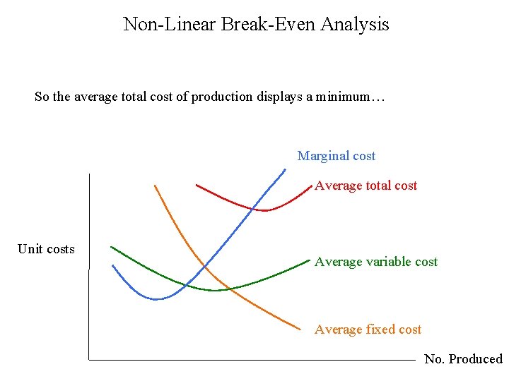
Non-Linear Break-Even Analysis So the average total cost of production displays a minimum… Marginal cost Average total cost Unit costs Average variable cost Average fixed cost No. Produced

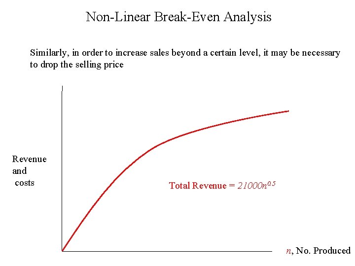
Non-Linear Break-Even Analysis Similarly, in order to increase sales beyond a certain level, it may be necessary to drop the selling price Revenue and costs Total Revenue = 21000 n 0. 5 n, No. Produced

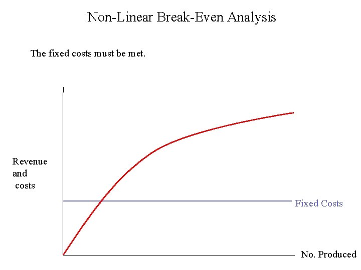
Non-Linear Break-Even Analysis The fixed costs must be met. Revenue and costs Fixed Costs No. Produced

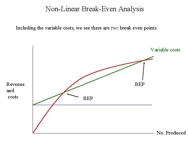
Non-Linear Break-Even Analysis Including the variable costs, we see there are two break even points Variable costs Revenue and costs BEP No. Produced

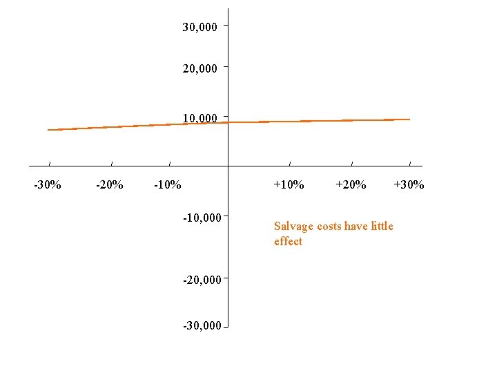
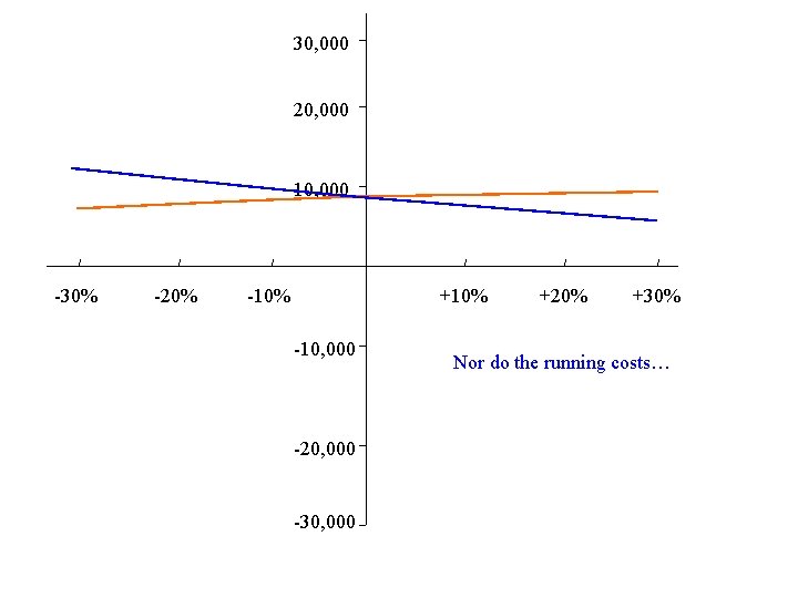
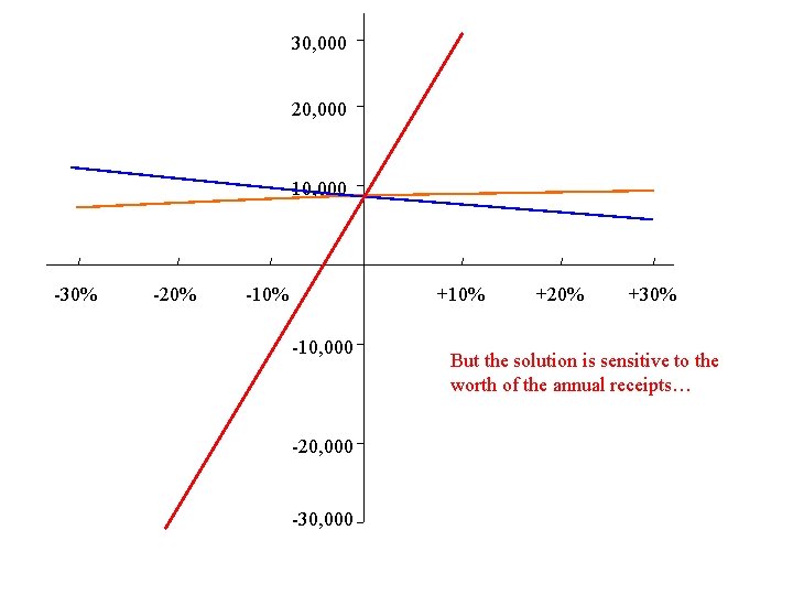
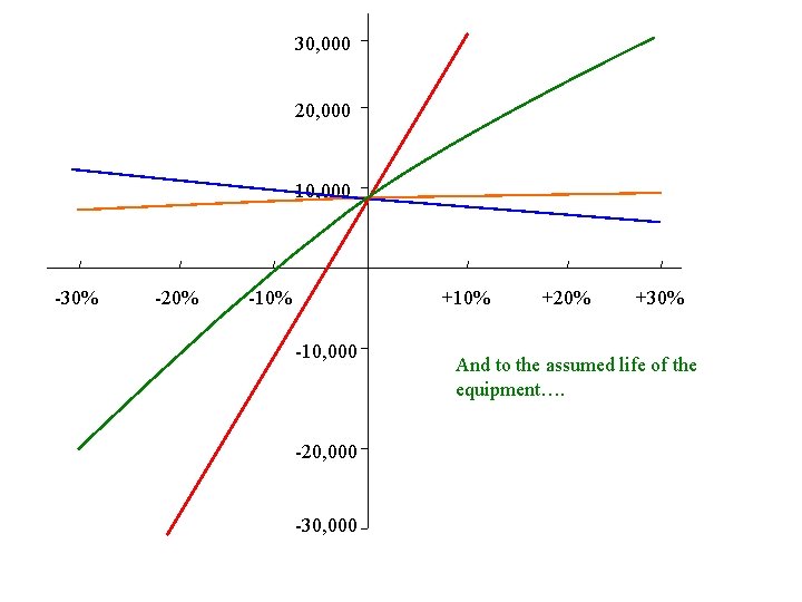
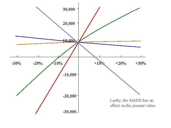
Sensitivity Analysis Having solved a problem, we determine the sensitivity of the solution to changes in the problem parameters. Hence we can decide whether and when to do further research. Example: a project has an initial cost of $170, 000 and is expected to yield annual receipts of $35, 000. There will be a salvage value of $20, 000 after ten years, and the annual operating cost will be $3, 000. If the MARR is 13%, should the investment be made?

30, 000 20, 000 10, 000 -30% -20% -10% +10% -10, 000 -20, 000 -30, 000 +20% Salvage costs have little effect +30%

30, 000 20, 000 10, 000 -30% -20% -10% +10% -10, 000 -20, 000 -30, 000 +20% +30% Nor do the running costs…

30, 000 20, 000 10, 000 -30% -20% -10% +10% -10, 000 -20, 000 -30, 000 +20% +30% But the solution is sensitive to the worth of the annual receipts…

30, 000 20, 000 10, 000 -30% -20% -10% +10% -10, 000 -20, 000 -30, 000 +20% +30% And to the assumed life of the equipment….

30, 000 20, 000 10, 000 -30% -20% -10% +20% +30% -10, 000 -20, 000 -30, 000 Lastly, the MARR has an effect on the present value.

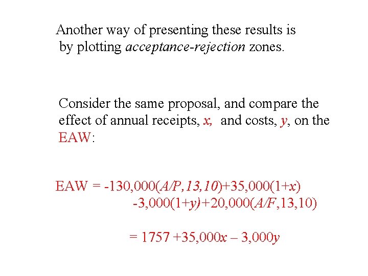
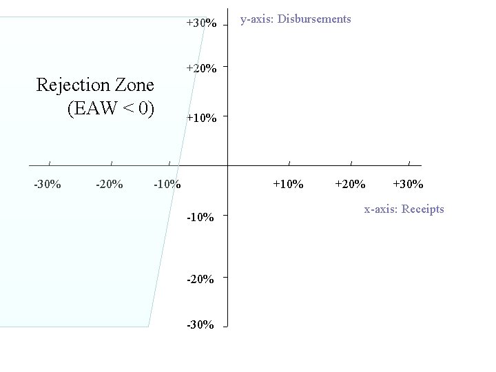
Another way of presenting these results is by plotting acceptance-rejection zones. Consider the same proposal, and compare the effect of annual receipts, x, and costs, y, on the EAW: EAW = -130, 000(A/P, 13, 10)+35, 000(1+x) -3, 000(1+y)+20, 000(A/F, 13, 10) = 1757 +35, 000 x – 3, 000 y

+30% Rejection Zone (EAW < 0) -30% -20% y-axis: Disbursements +20% +10% -10% -20% -30% +20% +30% x-axis: Receipts

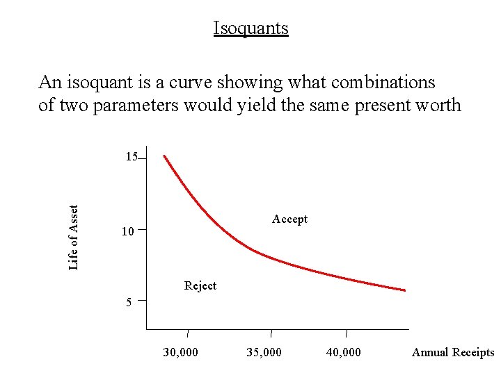
Isoquants An isoquant is a curve showing what combinations of two parameters would yield the same present worth Life of Asset 15 Accept 10 Reject 5 30, 000 35, 000 40, 000 Annual Receipts

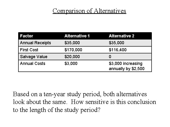
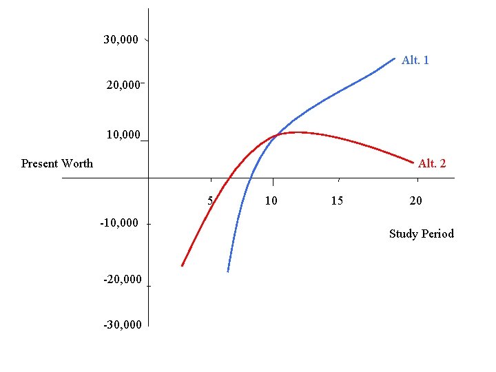
Comparison of Alternatives Factor Alternative 1 Alternative 2 Annual Receipts $35, 000 First Cost $170, 000 $116, 400 Salvage Value $20, 000 0 Annual Costs $3, 000 increasing annually by $2, 500 Based on a ten-year study period, both alternatives look about the same. How sensitive is this conclusion to the length of the study period?

30, 000 Alt. 1 20, 000 10, 000 Present Worth Alt. 2 5 -10, 000 -20, 000 -30, 000 10 15 20 Study Period

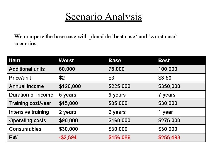
Scenario Analysis …also sometimes known as the `Goldilocks’ method…

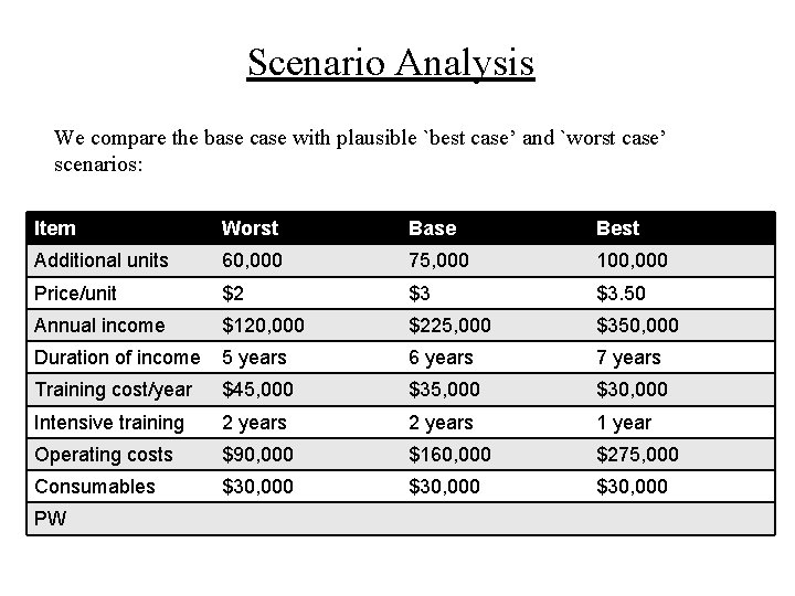
Scenario Analysis We compare the base case with plausible `best case’ and `worst case’ scenarios: Item Worst Base Best Additional units 60, 000 75, 000 100, 000 Price/unit $2 $3 $3. 50 Annual income $120, 000 $225, 000 $350, 000 Duration of income 5 years 6 years 7 years Training cost/year $45, 000 $30, 000 Intensive training 2 years 1 year Operating costs $90, 000 $160, 000 $275, 000 Consumables $30, 000 PW

Scenario Analysis We compare the base case with plausible `best case’ and `worst case’ scenarios: Item Worst Base Best Additional units 60, 000 75, 000 100, 000 Price/unit $2 $3 $3. 50 Annual income $120, 000 $225, 000 $350, 000 Duration of income 5 years 6 years 7 years Training cost/year $45, 000 $30, 000 Intensive training 2 years 1 year Operating costs $90, 000 $160, 000 $275, 000 Consumables $30, 000 PW -$2, 594 $156, 086 $255, 493