CSXXXAlgorithms X Lecture X Fibonacci Heaps CS XXX

CSXXX-Algorithms X Lecture X Fibonacci Heaps CS XXX Lecture X

Fibonacci Heaps • Binomial heaps support the mergeable heap operations (INSERT, MINIMUM, EXTRACT_MIN, UNION plus, DECREASE_KEY and DELETE) in O(lgn) worst-case time. • Fibonacci heaps support the mergeable heap operations that do not involve deleting an element in O(1) amortized time. CS XXX Lecture X 2

Fibonacci Heaps • Fibonacci heaps are especially desirable when the number of EXTRACT-MIN and DELETE operations is small relative to the number of other operations. • Fibonacci heaps are loosely based on binomial heaps. • A collection of trees if neither DECREASEKEY nor DELETE is ever invoked. • Each tree is like a binomial tree. CS XXX Lecture X 3

Fibonacci Heaps • Fibonacci heaps differ from binomial-heaps, however, in that they have more relaxed structure allowing for improved asymptotic time bounds work that maintains the structure is delayed until it is convenient to perform. • Like a binomial heap, a fibonacci heap is a collection of heap-ordered trees however, trees are not constrained to be binomial trees. • Trees within fibonacci heaps are rooted but unordered. CS XXX Lecture X 4

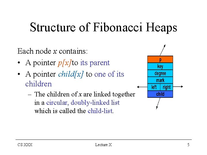
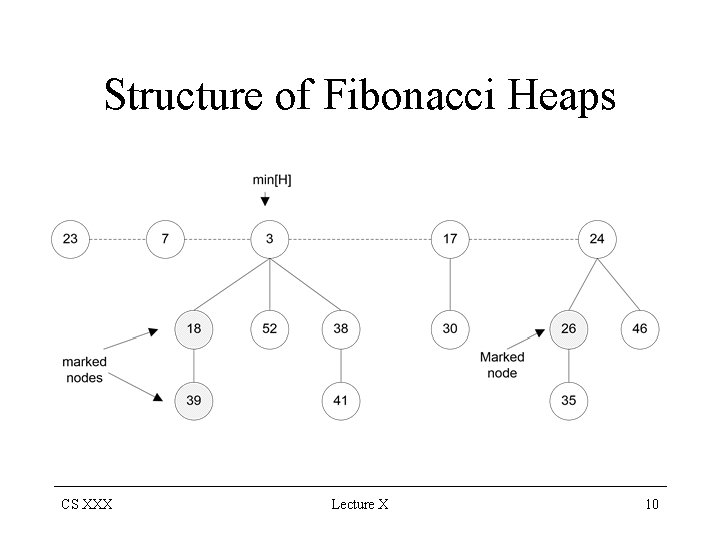
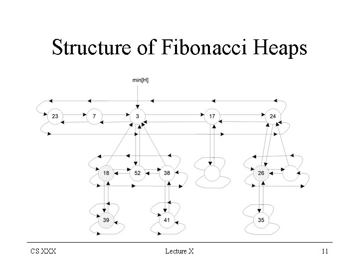
Structure of Fibonacci Heaps Each node x contains: • A pointer p[x]to its parent • A pointer child[x] to one of its children – The children of x are linked together in a circular, doubly-linked list which is called the child-list. CS XXX Lecture X 5

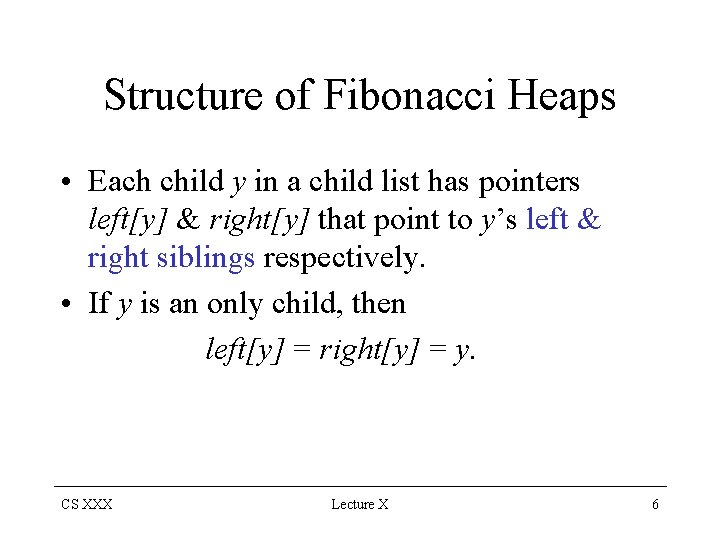
Structure of Fibonacci Heaps • Each child y in a child list has pointers left[y] & right[y] that point to y’s left & right siblings respectively. • If y is an only child, then left[y] = right[y] = y. CS XXX Lecture X 6

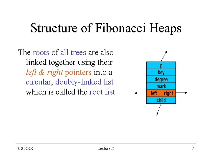
Structure of Fibonacci Heaps The roots of all trees are also linked together using their left & right pointers into a circular, doubly-linked list which is called the root list. CS XXX Lecture X 7

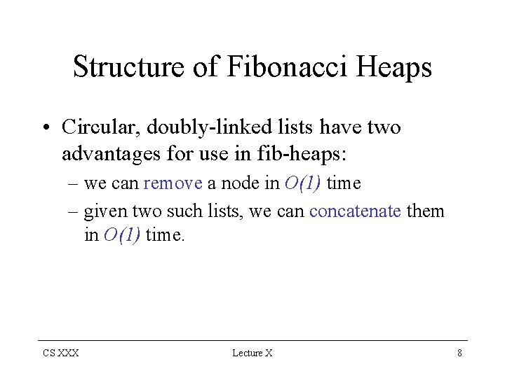
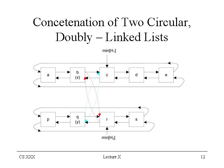
Structure of Fibonacci Heaps • Circular, doubly-linked lists have two advantages for use in fib-heaps: – we can remove a node in O(1) time – given two such lists, we can concatenate them in O(1) time. CS XXX Lecture X 8

Structure of Fibonacci Heaps • Two other fields in each node x – degreee[x]: the number of children in the child list of x – mark[x]: a boolean-valued field • indicates whether node x has lost a child since the last time x was made the child of another one • newly created nodes are unmarked • A node x becomes unmarked whenever it is made the child of another node CS XXX Lecture X 9

Structure of Fibonacci Heaps CS XXX Lecture X 10

Structure of Fibonacci Heaps CS XXX Lecture X 11

Concetenation of Two Circular, Doubly – Linked Lists CS XXX Lecture X 12

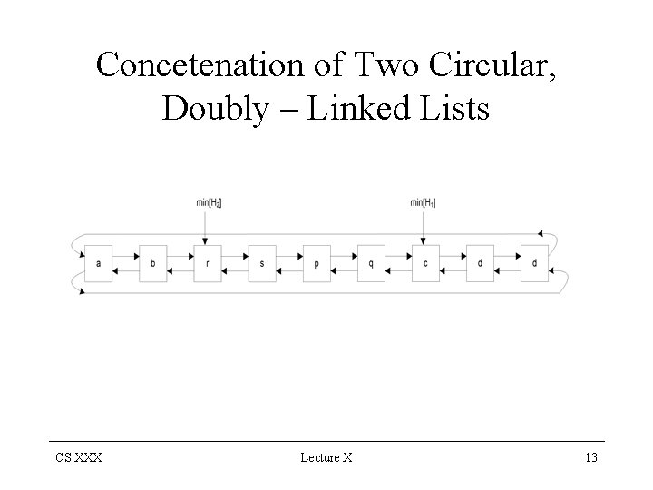
Concetenation of Two Circular, Doubly – Linked Lists CS XXX Lecture X 13

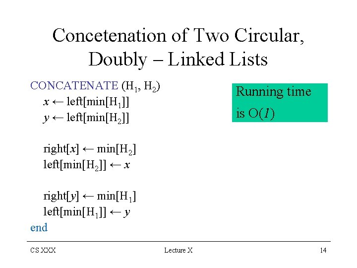
Concetenation of Two Circular, Doubly – Linked Lists CONCATENATE (H 1, H 2) x ← left[min[H 1]] y ← left[min[H 2]] Running time is O(1) right[x] ← min[H 2] left[min[H 2]] ← x right[y] ← min[H 1] left[min[H 1]] ← y end CS XXX Lecture X 14

Potential Function • A given fibonacci heap H – t(H): the number of trees in root list of H – m(H): the number of marked nodes in H • The potential of fibonacci heap H is: Φ(H) = t(H) + 2 m(H) • A fibonacci heap application begins with an empty heap: the initial potential = 0 • The potential is non-negative at all subsequent times. CS XXX Lecture X 15

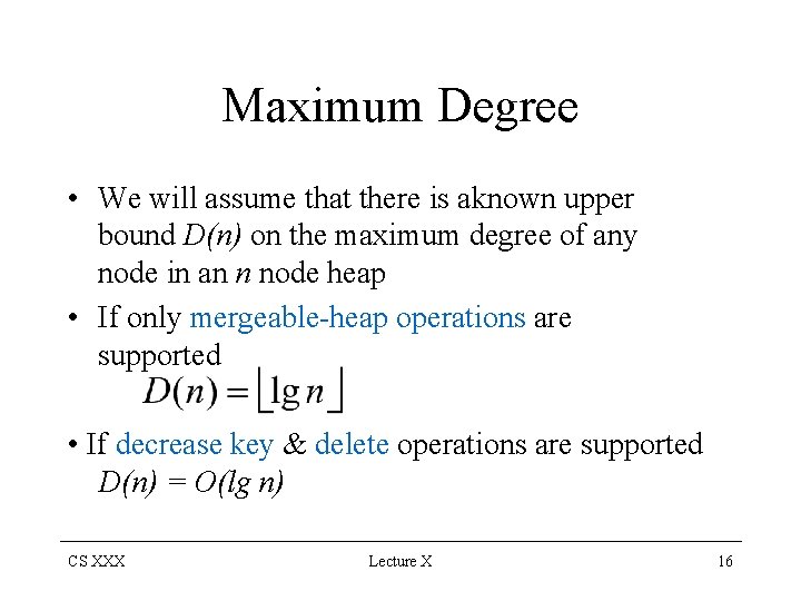
Maximum Degree • We will assume that there is aknown upper bound D(n) on the maximum degree of any node in an n node heap • If only mergeable-heap operations are supported • If decrease key & delete operations are supported D(n) = O(lg n) CS XXX Lecture X 16

Mergeable Heap Operations MAKE-HEAP, INSERT, MINIMUM, EXTRACT-MIN, UNION If only these operations are to be supported, each fibonacci-heap is a collection of unordered binomial trees. CS XXX Lecture X 17

Mergeable Heap Operations • An unordered binomial tree Uk – is like a binomial tree – defined recursively: • U 0 consists of a single node • Uk consists of two Uk-1’s for which the root of one is made into any child of the root of the other CS XXX Lecture X 18

Mergeable Heap Operations • Lemma which gives properties of binomial trees holds for unordered binomial trees as well but with the following variation on property 4 • Property 4’: For the unordered binomial tree Uk: – The root has degree k > the degree of any other node – The children of the root are the roots of subtrees U 0, U 1, . . , Uk-1 in some order CS XXX Lecture X 19

Mergeable Heap Operations • The key idea in the mergeable heap operations on fibonacci heaps is to delay work as long as possible. • Performance trade-off among implementations of the various operations: – If the number of trees is small we can quickly determine the new min node during EXTRACT-MIN – However we pay a price for ensuring that the number of trees is small CS XXX Lecture X 20

Mergeable Heap Operations • However we pay a price for ensuring that the number of trees is small • However it can take up to Ω(lg n) time – to insert a node into a binomial heap – or to unite two binomial heaps • We do not consolidate trees in a fibonacci heap when we insert a new node or unite two heaps • We delay the consolidation for the EXTRACTMIN operation when we really need to find the new minimum node. CS XXX Lecture X 21

Mergeable Heap Operations Creating a new fibonacci heap: MAKE-FIB-HEAP procedure – allocates and returns the fibonacci heap object H – Where n[H] = 0 and min[H] = NIL – There are no trees in the heap because t(H) = 0 and m(H) = 0 => Φ(H) = 0 the amortized cost = O(1) = the actual cost CS XXX Lecture X 22

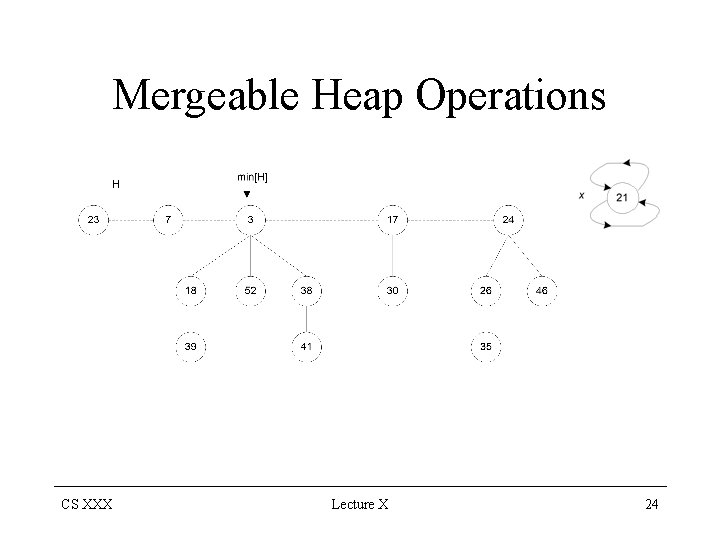
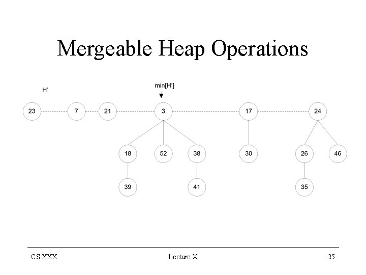
Mergeable Heap Operations Inserting a node FIB-HEAP-INSERT(H, x) degree[x] ← 0 p[x] ← NIL child[x] ← NIL left[x] ← x right[x] ← x mark[x] ← FALSE concatenate the root list containing x with root list H if key[x] < key[min[H]] then min[H] ← x endif n[H] ← n[H] + 1 end CS XXX Lecture X 23

Mergeable Heap Operations CS XXX Lecture X 24

Mergeable Heap Operations CS XXX Lecture X 25

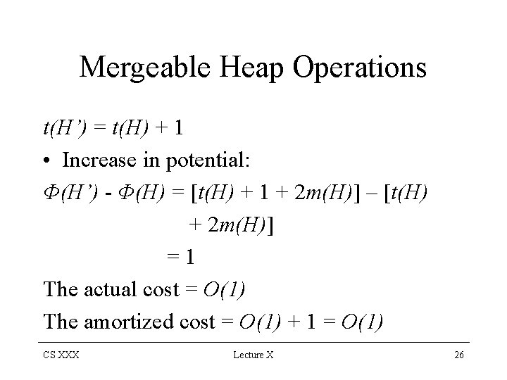
Mergeable Heap Operations t(H’) = t(H) + 1 • Increase in potential: Φ(H’) - Φ(H) = [t(H) + 1 + 2 m(H)] – [t(H) + 2 m(H)] =1 The actual cost = O(1) The amortized cost = O(1) + 1 = O(1) CS XXX Lecture X 26

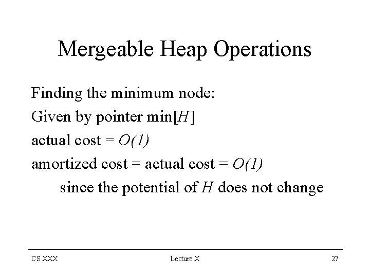
Mergeable Heap Operations Finding the minimum node: Given by pointer min[H] actual cost = O(1) amortized cost = actual cost = O(1) since the potential of H does not change CS XXX Lecture X 27

Uniting Two Fibonacci Heaps FIB-HEAP-UNION(H 1, H 2) H = MAKE-FIB-HEAP() if key[min[H 1]] ≤ key[min[H 2]] then min[H] ← min[H 1] else min[H] ← min[H 2] endif concatenate the root lists of H 1 and H 2 n[H] ← n[H 1] + n[H 2] Free the objects H 1 and H 2 return H end CS XXX Lecture X 28

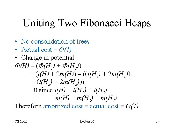
Uniting Two Fibonacci Heaps • No consolidation of trees • Actual cost = O(1) • Change in potential Φ(H) – (Φ(H 1) + Φ(H 2)) = = (t(H) + 2 m(H)) – ((t(H 1) + 2 m(H 1)) + (t(H 2) + 2 m(H 2))) = 0 since t(H) = t(H 1) + t(H 2) m(H) = m(H 1) + m(H 2) Therefore amortized cost = actual cost = O(1) CS XXX Lecture X 29

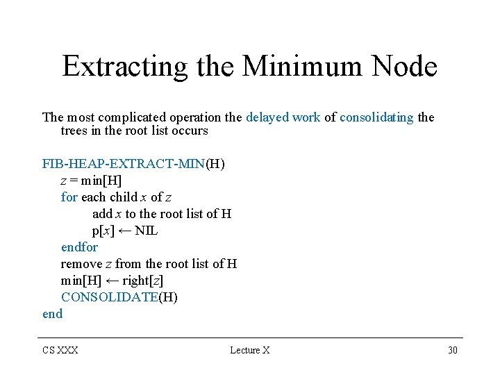
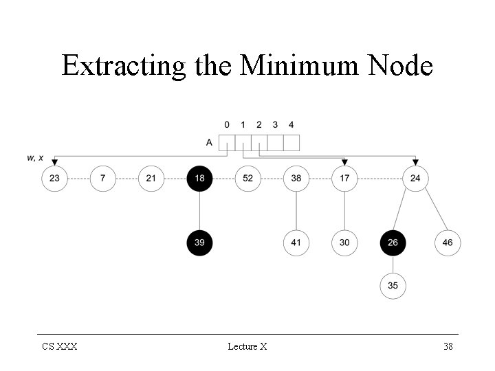
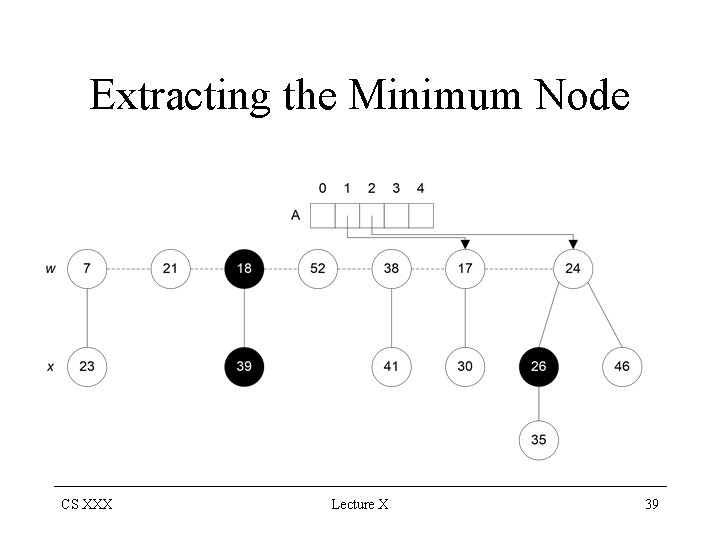
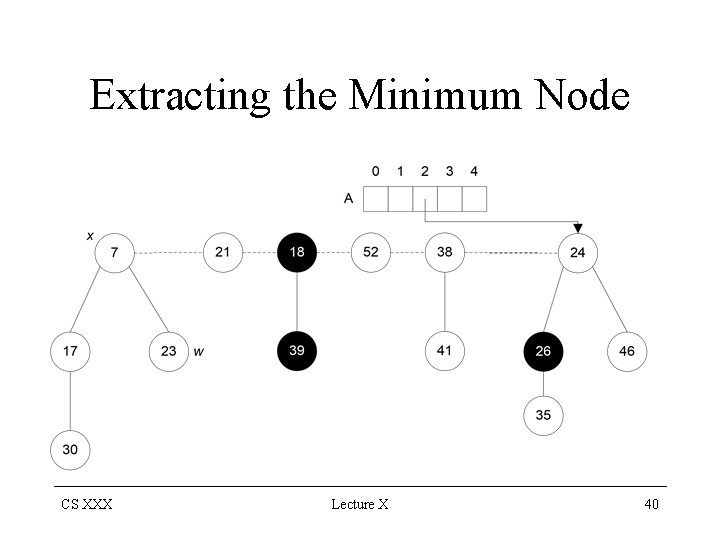
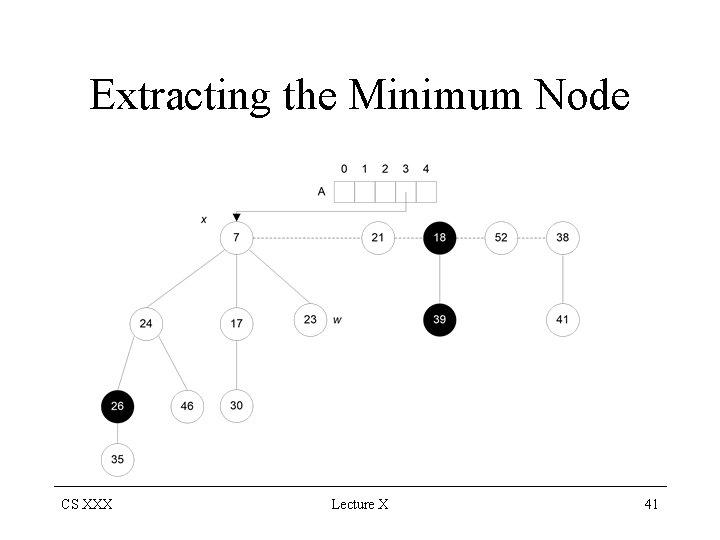
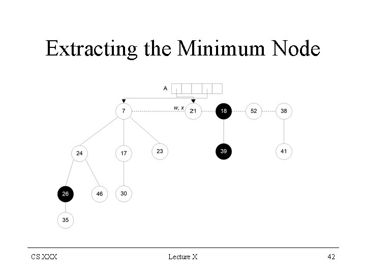
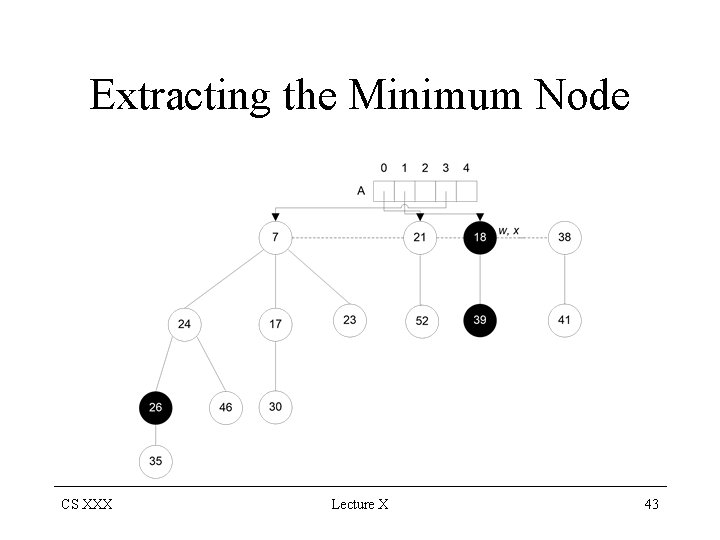
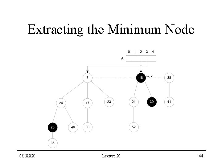
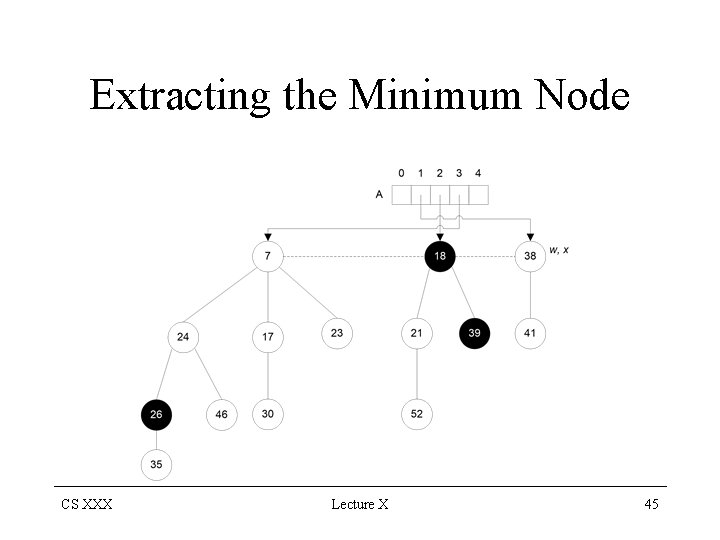
Extracting the Minimum Node The most complicated operation the delayed work of consolidating the trees in the root list occurs FIB-HEAP-EXTRACT-MIN(H) z = min[H] for each child x of z add x to the root list of H p[x] ← NIL endfor remove z from the root list of H min[H] ← right[z] CONSOLIDATE(H) end CS XXX Lecture X 30

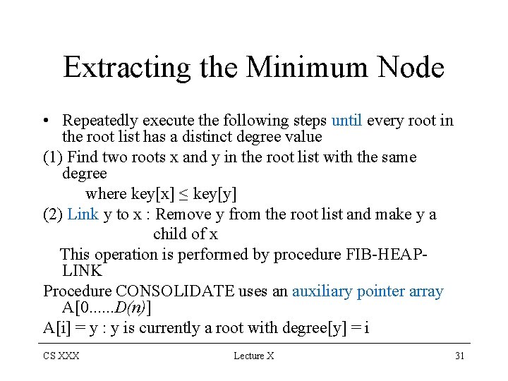
Extracting the Minimum Node • Repeatedly execute the following steps until every root in the root list has a distinct degree value (1) Find two roots x and y in the root list with the same degree where key[x] ≤ key[y] (2) Link y to x : Remove y from the root list and make y a child of x This operation is performed by procedure FIB-HEAPLINK Procedure CONSOLIDATE uses an auxiliary pointer array A[0. . . D(n)] A[i] = y : y is currently a root with degree[y] = i CS XXX Lecture X 31

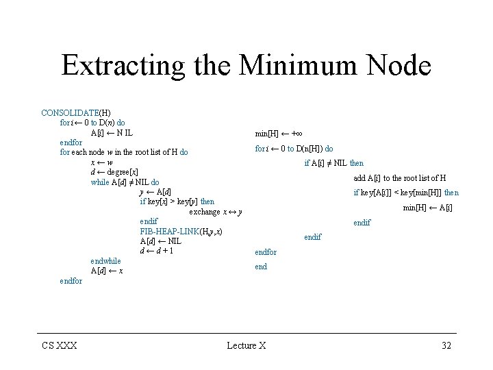
Extracting the Minimum Node CONSOLIDATE(H) for i← 0 to D(n) do A[i] ← N IL endfor each node w in the root list of H do x←w d ← degree[x] while A[d] ≠ NIL do y ← A[d] if key[x] > key[y] then exchange x ↔ y endif FIB-HEAP-LINK(H, y, x) A[d] ← NIL d←d+1 endwhile A[d] ← x endfor CS XXX min[H] ← +∞ for i ← 0 to D(n[H]) do if A[i] ≠ NIL then add A[i] to the root list of H if key[A[i]] < key[min[H]] then min[H] ← A[i] endif endfor end Lecture X 32

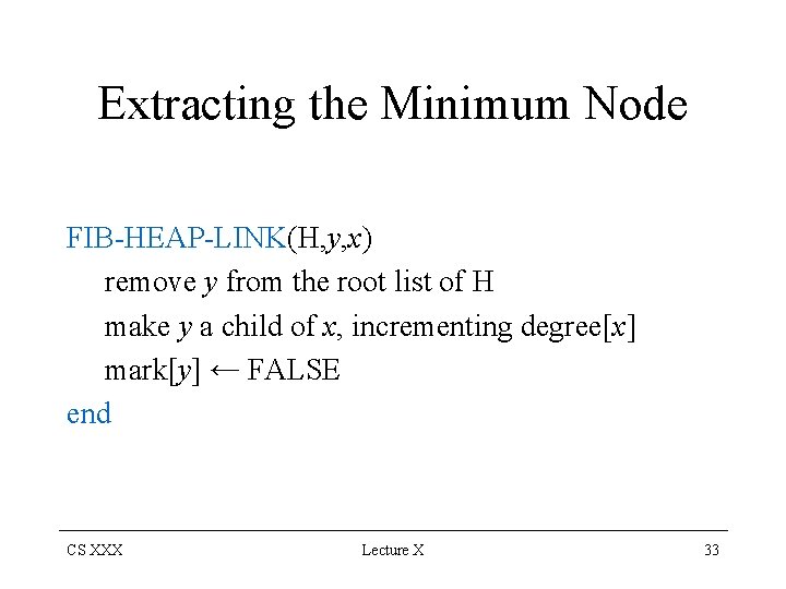
Extracting the Minimum Node FIB-HEAP-LINK(H, y, x) remove y from the root list of H make y a child of x, incrementing degree[x] mark[y] ← FALSE end CS XXX Lecture X 33

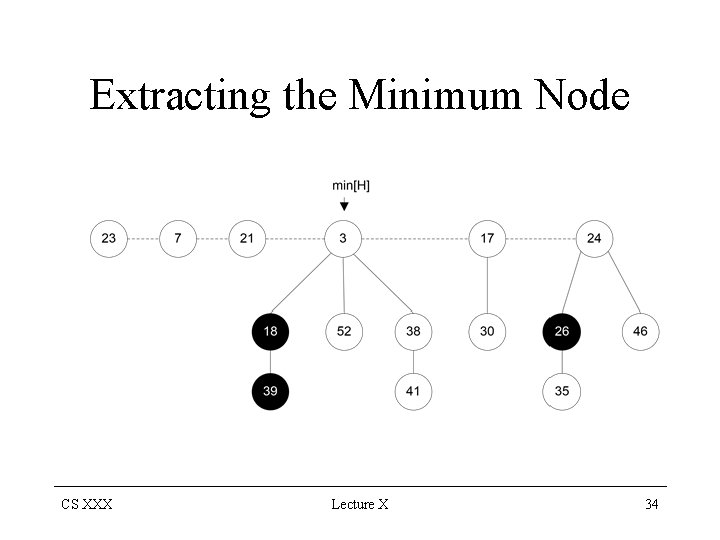
Extracting the Minimum Node CS XXX Lecture X 34

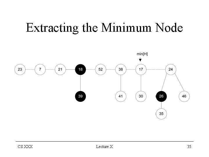
Extracting the Minimum Node CS XXX Lecture X 35

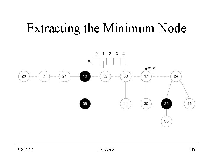
Extracting the Minimum Node CS XXX Lecture X 36

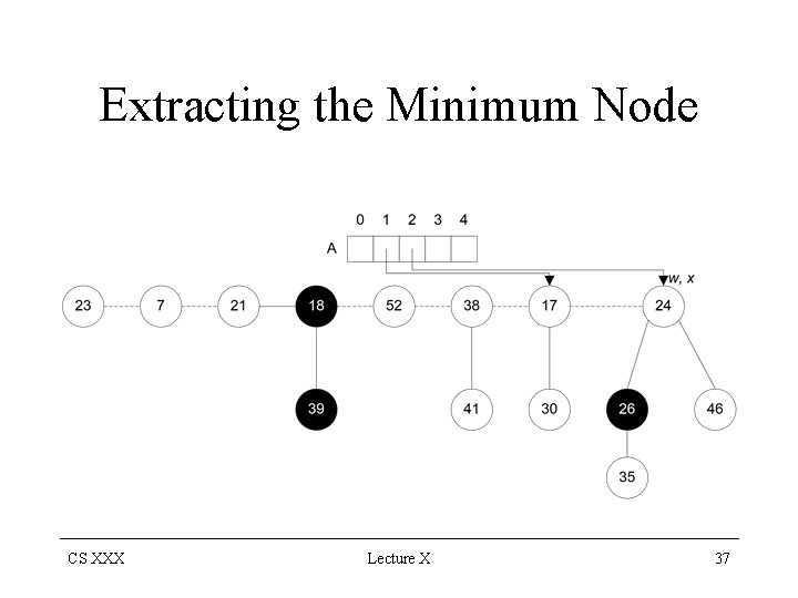
Extracting the Minimum Node CS XXX Lecture X 37

Extracting the Minimum Node CS XXX Lecture X 38

Extracting the Minimum Node CS XXX Lecture X 39

Extracting the Minimum Node CS XXX Lecture X 40

Extracting the Minimum Node CS XXX Lecture X 41

Extracting the Minimum Node CS XXX Lecture X 42

Extracting the Minimum Node CS XXX Lecture X 43

Extracting the Minimum Node CS XXX Lecture X 44

Extracting the Minimum Node CS XXX Lecture X 45

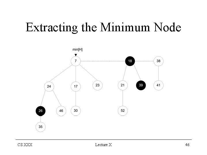
Extracting the Minimum Node CS XXX Lecture X 46

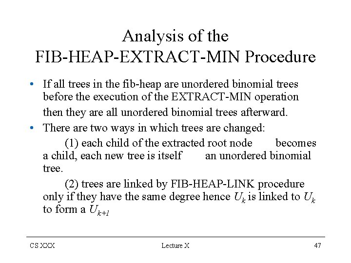
Analysis of the FIB-HEAP-EXTRACT-MIN Procedure • If all trees in the fib-heap are unordered binomial trees before the execution of the EXTRACT-MIN operation they are all unordered binomial trees afterward. • There are two ways in which trees are changed: (1) each child of the extracted root node becomes a child, each new tree is itself an unordered binomial tree. (2) trees are linked by FIB-HEAP-LINK procedure only if they have the same degree hence Uk is linked to Uk to form a Uk+1 CS XXX Lecture X 47

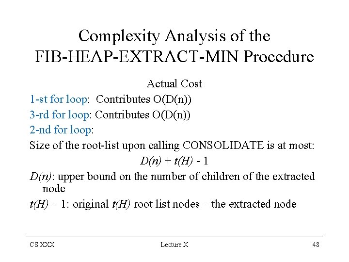
Complexity Analysis of the FIB-HEAP-EXTRACT-MIN Procedure Actual Cost 1 -st for loop: Contributes O(D(n)) 3 -rd for loop: Contributes O(D(n)) 2 -nd for loop: Size of the root-list upon calling CONSOLIDATE is at most: D(n) + t(H) - 1 D(n): upper bound on the number of children of the extracted node t(H) – 1: original t(H) root list nodes – the extracted node CS XXX Lecture X 48

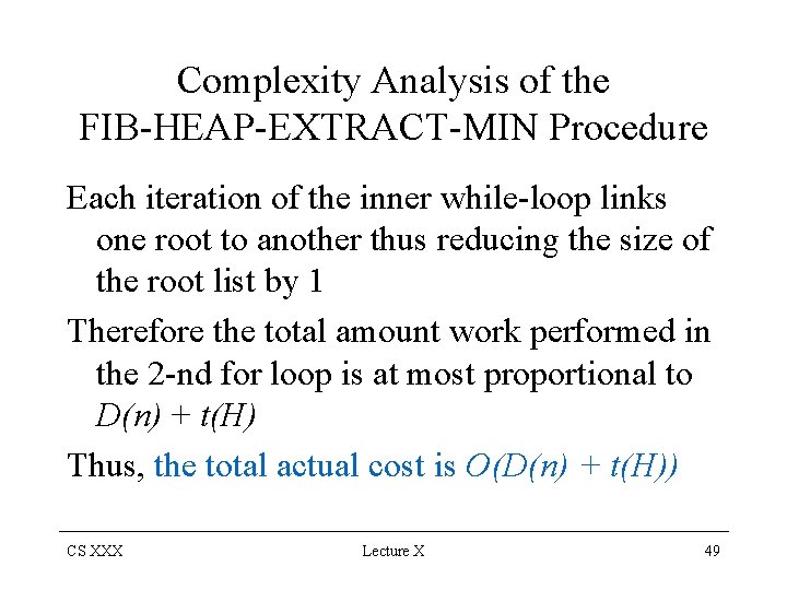
Complexity Analysis of the FIB-HEAP-EXTRACT-MIN Procedure Each iteration of the inner while-loop links one root to another thus reducing the size of the root list by 1 Therefore the total amount work performed in the 2 -nd for loop is at most proportional to D(n) + t(H) Thus, the total actual cost is O(D(n) + t(H)) CS XXX Lecture X 49

Complexity Analysis of the FIB-HEAP-EXTRACT-MIN Procedure Amortized Cost Potential before: t(H) + 2 m(H) Potential after: at most (D(n) + 1)+2 m(H) since at most D(n)+1 roots remain & no nodes marked Amortized cost = O(D(n) + t(H)) + [(D(n) + 1) + 2 m(H)] – [t(H) + 2 m(H)] = O(D(n)) + O(t(H)) – D(n) – t(H) = O(D(n)) CS XXX Lecture X 50

Complexity Analysis of the FIB-HEAP-EXTRACT-MIN Procedure The cost of performing each link is paid for by the reduction in potential due to the link reducing the number of roots by one CS XXX Lecture X 51

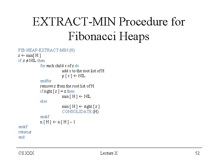
EXTRACT-MIN Procedure for Fibonacci Heaps FIB-HEAP-EXTRACT-MIN (H) z min[ H ] if z ≠ NIL then for each child x of z do add x to the root list of H p [ x ] NIL endfor remove z from the root list of H if right [ z ] = z then min [ H ] NIL else min [ H ] right [ z ] CONSOLIDATE (H) endif n[H]– 1 endif return z end CS XXX Lecture X 52

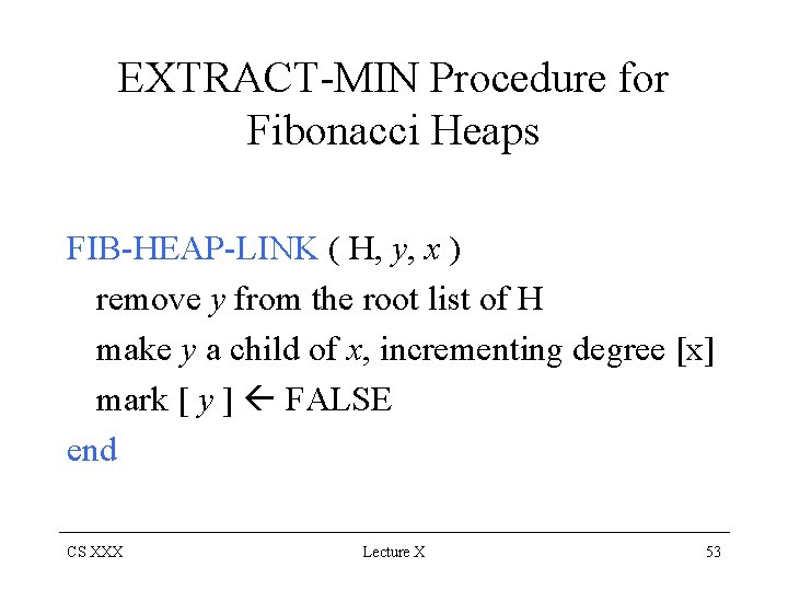
EXTRACT-MIN Procedure for Fibonacci Heaps FIB-HEAP-LINK ( H, y, x ) remove y from the root list of H make y a child of x, incrementing degree [x] mark [ y ] FALSE end CS XXX Lecture X 53

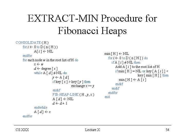
EXTRACT-MIN Procedure for Fibonacci Heaps CONSOLIDATE ( H ) for i 0 to D ( n ( H ) ) A[ i ] NIL endfor each node w in the root list of H do x w d degree [ x ] while A [ d ] ≠ NIL do y A[d] if key [ x ] > key [ y ] then exchange x ↔ y endif FIB-HEAP-LINK ( H , y, x ) A [ d ] NIL d d+1 endwhile A[d] x endfor CS XXX Lecture X min [ H ] NIL for i 0 to D ( n [ H ] ) do if A [ i ] ≠ NIL then Add A [ i ] to the root list of H if min [ H ] = NIL or key [ A [ i ] ] < key [ min [ H ] ] then min [ H ] A [ i ] endif endfor end 54

Bounding the Maximum Degree For each node x within a fibonacci heap, define size(x): the number of nodes, including itself, in the subtree rooted at x NOTE: x need not to be in the root list, it can be any node at all. We shall show that size(x) is exponential in degree[x] CS XXX Lecture X 55

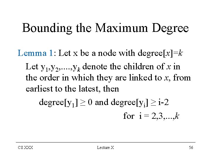
Bounding the Maximum Degree Lemma 1: Let x be a node with degree[x]=k Let y 1, y 2, . . , yk denote the children of x in the order in which they are linked to x, from earliest to the latest, then degree[y 1] ≥ 0 and degree[yi] ≥ i-2 for i = 2, 3, . . . , k CS XXX Lecture X 56

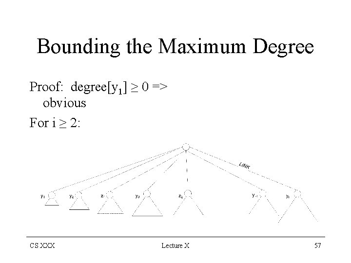
Bounding the Maximum Degree Proof: degree[y 1] ≥ 0 => obvious For i ≥ 2: CS XXX Lecture X 57

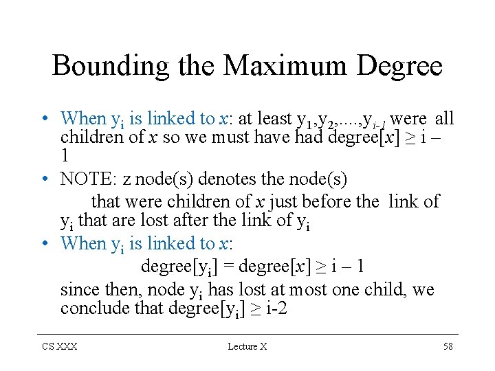
Bounding the Maximum Degree • When yi is linked to x: at least y 1, y 2, . . , yi-1 were all children of x so we must have had degree[x] ≥ i – 1 • NOTE: z node(s) denotes the node(s) that were children of x just before the link of yi that are lost after the link of yi • When yi is linked to x: degree[yi] = degree[x] ≥ i – 1 since then, node yi has lost at most one child, we conclude that degree[yi] ≥ i-2 CS XXX Lecture X 58

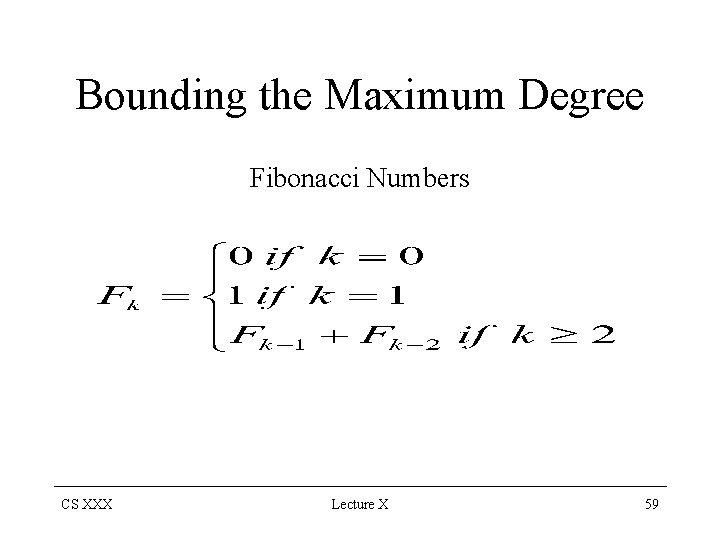
Bounding the Maximum Degree Fibonacci Numbers CS XXX Lecture X 59

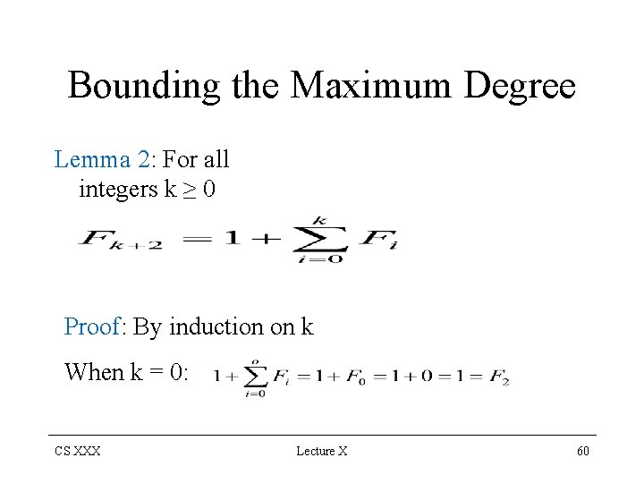
Bounding the Maximum Degree Lemma 2: For all integers k ≥ 0 Proof: By induction on k When k = 0: CS XXX Lecture X 60

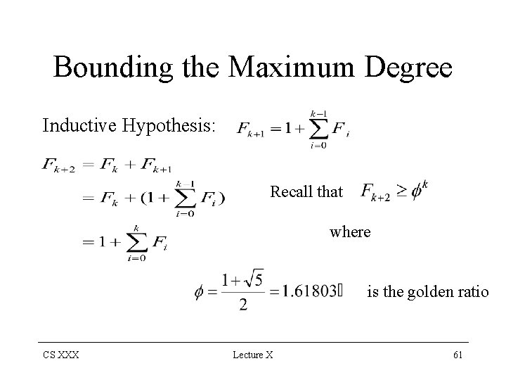
Bounding the Maximum Degree Inductive Hypothesis: Recall that where is the golden ratio CS XXX Lecture X 61

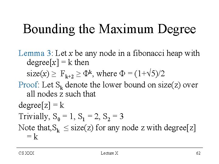
Bounding the Maximum Degree Lemma 3: Let x be any node in a fibonacci heap with degree[x] = k then size(x) ≥ Fk+2 ≥ Φk, where Φ = (1+√ 5)/2 Proof: Let Sk denote the lower bound on size(z) over all nodes z such that degree[z] = k Trivially, S 0 = 1, S 1 = 2, S 2 = 3 Note that, Sk ≤ size(z) for any node z with degree[z] =k CS XXX Lecture X 62

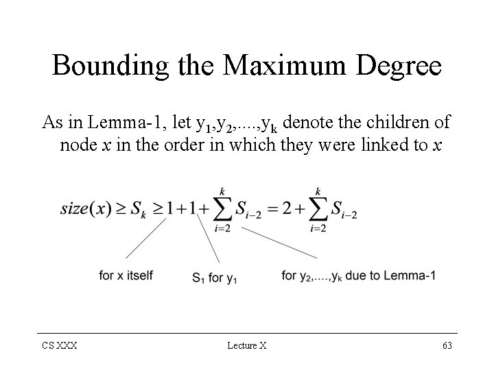
Bounding the Maximum Degree As in Lemma-1, let y 1, y 2, . . , yk denote the children of node x in the order in which they were linked to x CS XXX Lecture X 63

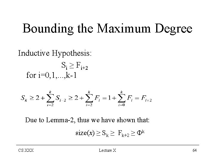
Bounding the Maximum Degree Inductive Hypothesis: Si ≥ Fi+2 for i=0, 1, . . . , k-1 Due to Lemma-2, thus we have shown that: size(x) ≥ Sk ≥ Fk+2 ≥ Φk CS XXX Lecture X 64

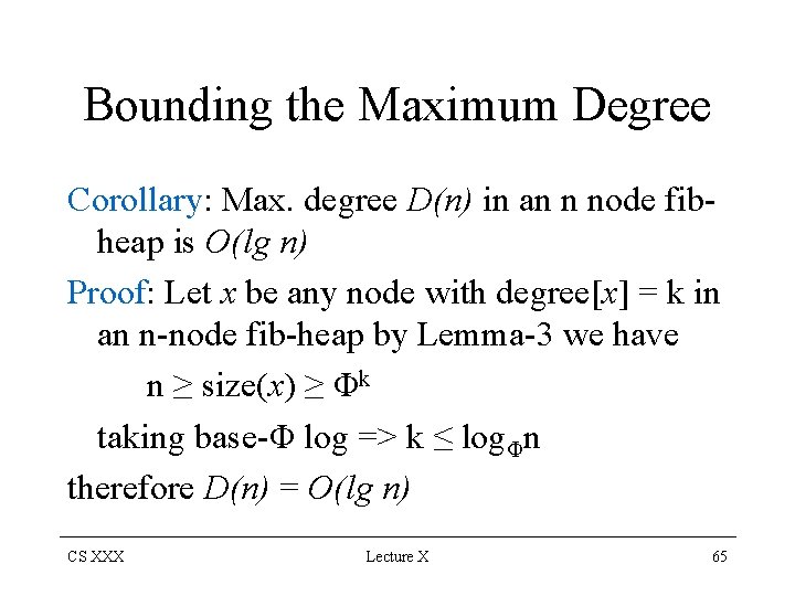
Bounding the Maximum Degree Corollary: Max. degree D(n) in an n node fibheap is O(lg n) Proof: Let x be any node with degree[x] = k in an n-node fib-heap by Lemma-3 we have n ≥ size(x) ≥ Φk taking base-Φ log => k ≤ logΦn therefore D(n) = O(lg n) CS XXX Lecture X 65

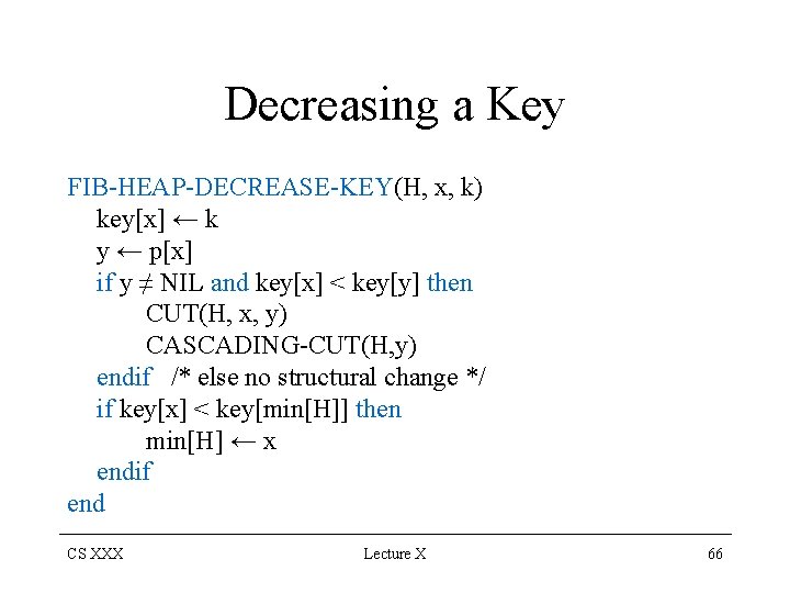
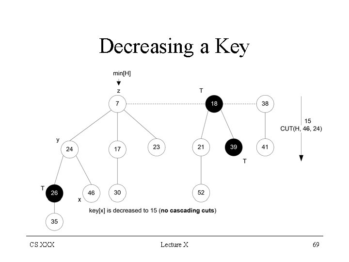
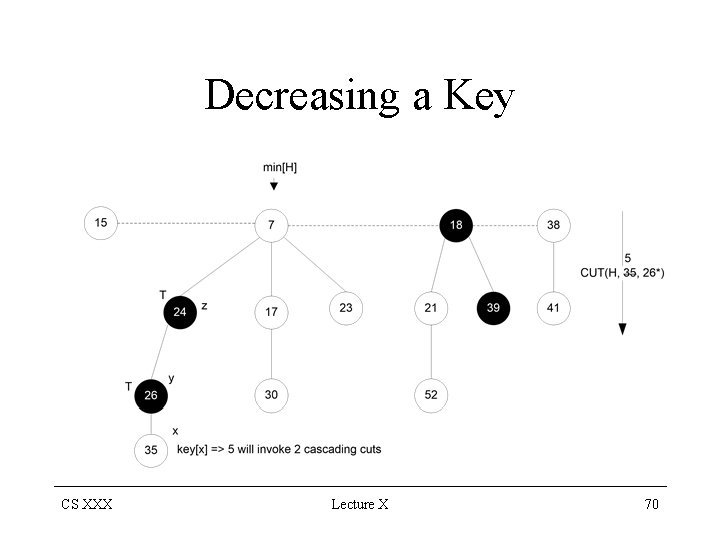
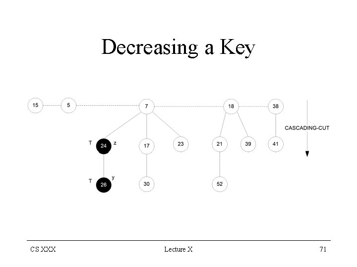
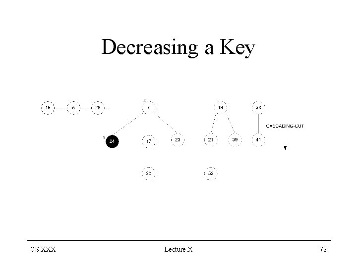
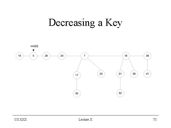
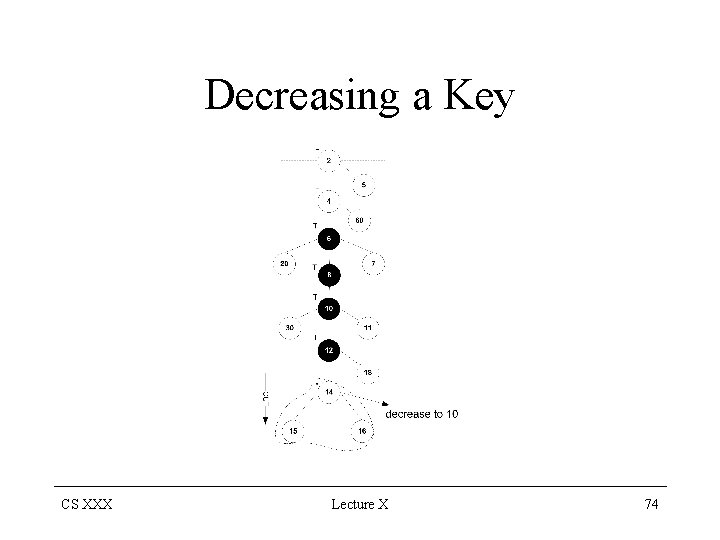
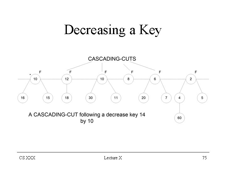
Decreasing a Key FIB-HEAP-DECREASE-KEY(H, x, k) key[x] ← k y ← p[x] if y ≠ NIL and key[x] < key[y] then CUT(H, x, y) CASCADING-CUT(H, y) endif /* else no structural change */ if key[x] < key[min[H]] then min[H] ← x endif end CS XXX Lecture X 66

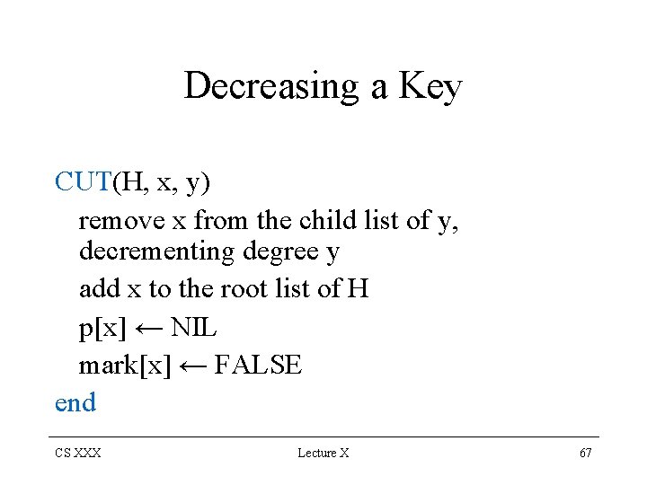
Decreasing a Key CUT(H, x, y) remove x from the child list of y, decrementing degree y add x to the root list of H p[x] ← NIL mark[x] ← FALSE end CS XXX Lecture X 67

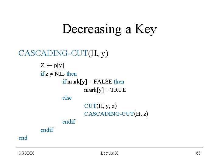
Decreasing a Key CASCADING-CUT(H, y) z ← p[y] if z ≠ NIL then if mark[y] = FALSE then mark[y] = TRUE else CUT(H, y, z) CASCADING-CUT(H, z) endif end CS XXX Lecture X 68

Decreasing a Key CS XXX Lecture X 69

Decreasing a Key CS XXX Lecture X 70

Decreasing a Key CS XXX Lecture X 71

Decreasing a Key CS XXX Lecture X 72

Decreasing a Key CS XXX Lecture X 73

Decreasing a Key CS XXX Lecture X 74

Decreasing a Key CS XXX Lecture X 75

Amortized Cost of FIB-HEAP-DECREASE-KEY Procedure Actual Cost O(1) time + the time required to perform the cascading cuts, suppose that CASCADINGCUT is recursively called c times each call takes O(1) time exclusive of recursive calls therefore, the actual cost = O(1) + O(c) = O(c) CS XXX Lecture X 76

Amortized Cost of FIB-HEAP-DECREASE-KEY Procedure Amortized Cost Let H denote the fib-heap prior to the DECREASE-KEY operation. Each recursive call of CASCADING-CUT, except for the last one, cuts a marked node and last call of cascading cut may mark a node. CS XXX Lecture X 77

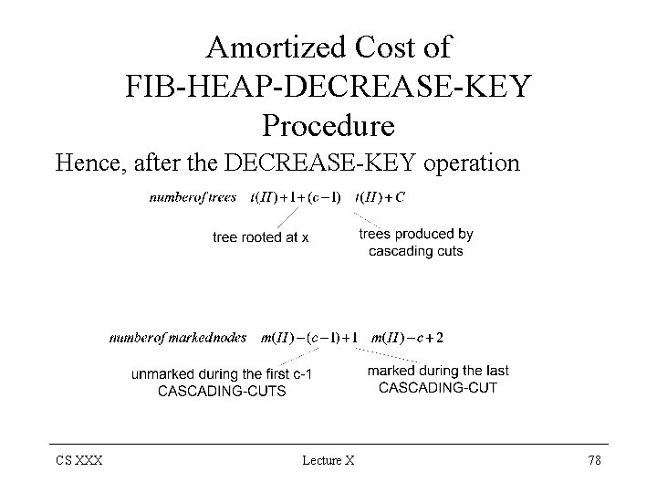
Amortized Cost of FIB-HEAP-DECREASE-KEY Procedure Hence, after the DECREASE-KEY operation CS XXX Lecture X 78

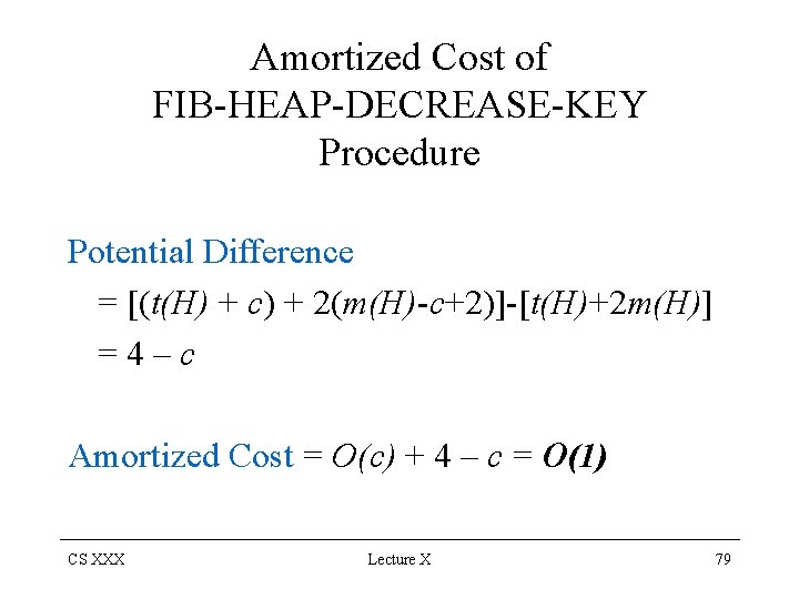
Amortized Cost of FIB-HEAP-DECREASE-KEY Procedure Potential Difference = [(t(H) + c) + 2(m(H)-c+2)]-[t(H)+2 m(H)] =4–c Amortized Cost = O(c) + 4 – c = O(1) CS XXX Lecture X 79

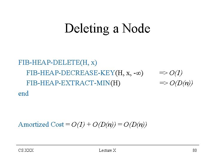
Deleting a Node FIB-HEAP-DELETE(H, x) FIB-HEAP-DECREASE-KEY(H, x, -∞) FIB-HEAP-EXTRACT-MIN(H) end => O(1) => O(D(n)) Amortized Cost = O(1) + O(D(n)) = O(D(n)) CS XXX Lecture X 80

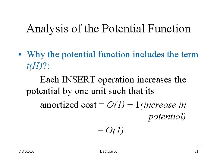
Analysis of the Potential Function • Why the potential function includes the term t(H)? : Each INSERT operation increases the potential by one unit such that its amortized cost = O(1) + 1(increase in potential) = O(1) CS XXX Lecture X 81

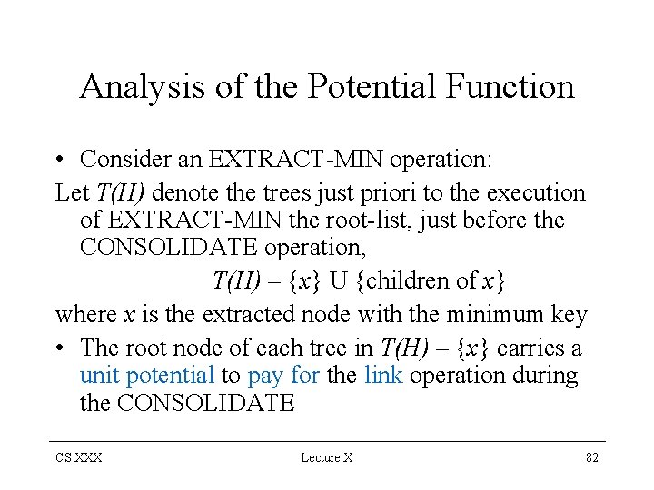
Analysis of the Potential Function • Consider an EXTRACT-MIN operation: Let T(H) denote the trees just priori to the execution of EXTRACT-MIN the root-list, just before the CONSOLIDATE operation, T(H) – {x} U {children of x} where x is the extracted node with the minimum key • The root node of each tree in T(H) – {x} carries a unit potential to pay for the link operation during the CONSOLIDATE CS XXX Lecture X 82

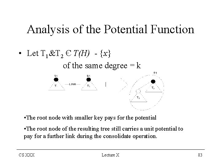
Analysis of the Potential Function • Let T 1&T 2 Є T(H) - {x} of the same degree = k • The root node with smaller key pays for the potential • The root node of the resulting tree still carries a unit potential to pay for a further link during the consolidate operation. CS XXX Lecture X 83

Analysis of the Potential Function • Why the potential function includes the term 2 m(H)? : – When a marked node y is cut by a cascading cut its mark bit is cleared so the potential is reduced by 2 – One unit pays for the cut and clearing the mark field – The other unit compensates for the unit increase in potential due to node y becoming a root CS XXX Lecture X 84

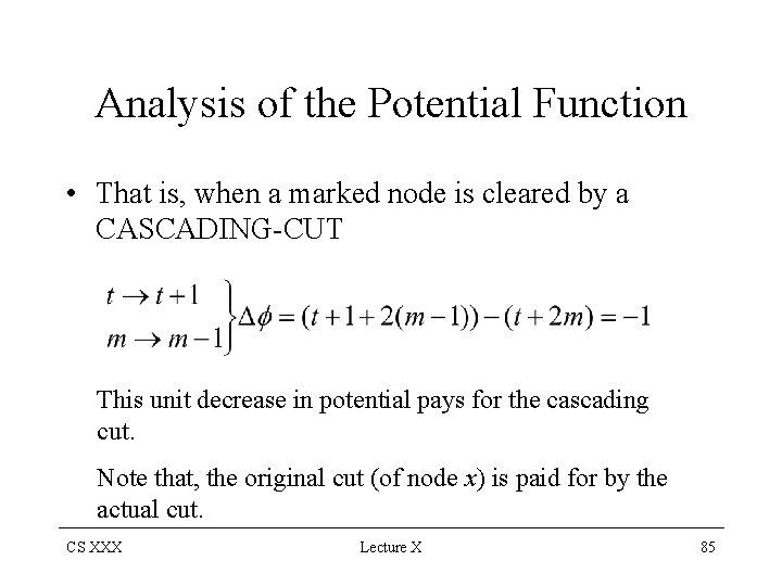
Analysis of the Potential Function • That is, when a marked node is cleared by a CASCADING-CUT This unit decrease in potential pays for the cascading cut. Note that, the original cut (of node x) is paid for by the actual cut. CS XXX Lecture X 85

Bounding the Maximum Degree • Why do we apply CASCADING-CUT during DECREASE-KEY operation? • To maintain the size of any tree/subtree exponential in the degree of its root node. e. g. : to prevent cases where size[x] = degree[x] + 1 CS XXX Lecture X 86

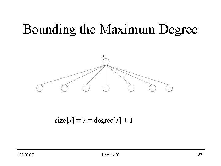
Bounding the Maximum Degree size[x] = 7 = degree[x] + 1 CS XXX Lecture X 87

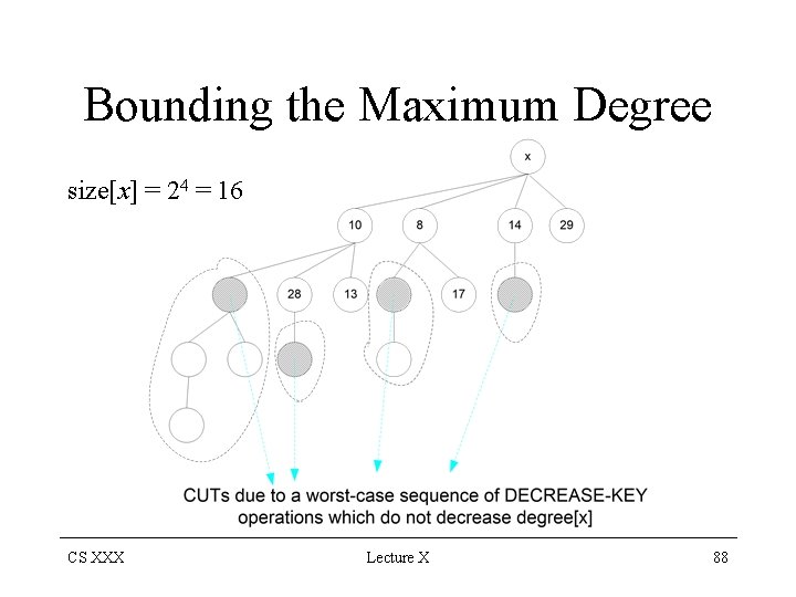
Bounding the Maximum Degree size[x] = 24 = 16 CS XXX Lecture X 88

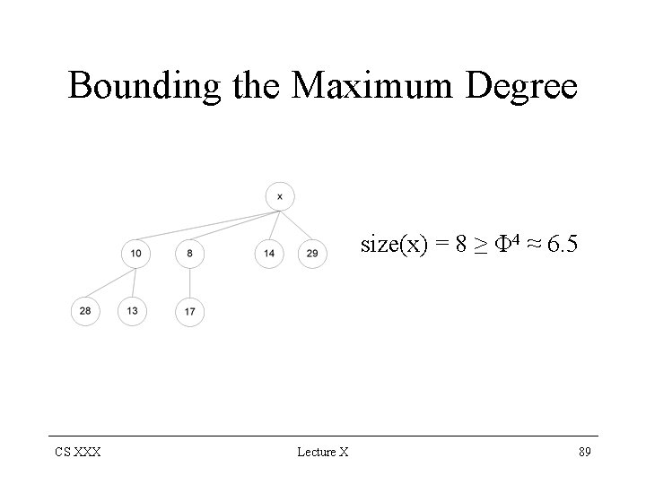
Bounding the Maximum Degree size(x) = 8 ≥ Φ 4 ≈ 6. 5 CS XXX Lecture X 89