CSI 5388 Functional Elements of Statistics for Machine

CSI 5388: Functional Elements of Statistics for Machine Learning Part II 1

Contents of the Lecture n Part I (This set of lecture notes): • Definition and Preliminaries • Hypothesis Testing: Parametric Approaches n Part II (The next set of lecture notes) • Hypothesis Testing: Non-Parametric Approaches • Power of a Test • Statistical Tests for Comparing Multiple Classifiers 2

Non-parametric approaches to Hypothesis testing n n The hypothesis testing procedures discussed in the previous lecture are called parametric. This means that they are based on assumptions regarding the distribution of the population for which the test was ran, and rely on the estimation of parameters from these distributions. In our cases, we assumed that the distributions were either normal or followed a Student t distribution. The parameters we estimated were the mean and the variance. The problem we now turn to is the issue of hypothesis testing that is not based on assumptions regarding the distribution and do not rely on the 3 estimation of parameters.

The Different Types of non-parametric hypothesis testing approaches I n There are two important families of tests that do not involve distributional assumptions and parameter estimations: • Nonparametric tests, which rely on ranking the data and performing a statistical test on the ranks. • Resampling statistics which consist of drawing samples repeatedly from a population and evaluating the distribution of the result. Resampling Statistics will be discussed in the next lecture. 4

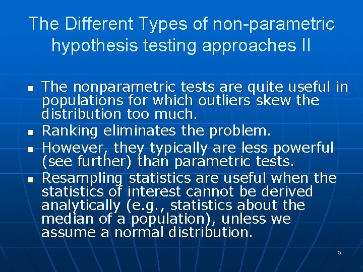
The Different Types of non-parametric hypothesis testing approaches II n n The nonparametric tests are quite useful in populations for which outliers skew the distribution too much. Ranking eliminates the problem. However, they typically are less powerful (see further) than parametric tests. Resampling statistics are useful when the statistics of interest cannot be derived analytically (e. g. , statistics about the median of a population), unless we assume a normal distribution. 5

Non-Parametric Tests Wilcoxon’s Rank-Sum Test n n The case of independent samples The case of matched pairs 6

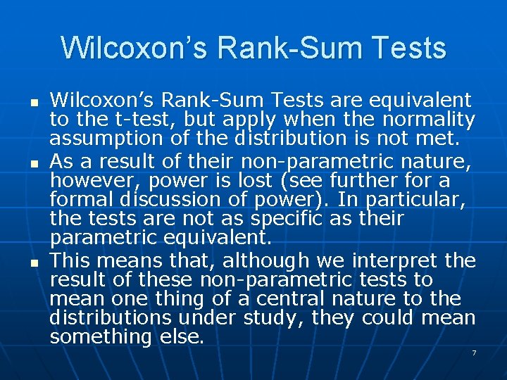
Wilcoxon’s Rank-Sum Tests n n n Wilcoxon’s Rank-Sum Tests are equivalent to the t-test, but apply when the normality assumption of the distribution is not met. As a result of their non-parametric nature, however, power is lost (see further for a formal discussion of power). In particular, the tests are not as specific as their parametric equivalent. This means that, although we interpret the result of these non-parametric tests to mean one thing of a central nature to the distributions under study, they could mean something else. 7

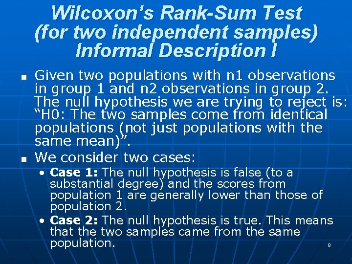
Wilcoxon’s Rank-Sum Test (for two independent samples) Informal Description I n n Given two populations with n 1 observations in group 1 and n 2 observations in group 2. The null hypothesis we are trying to reject is: “H 0: The two samples come from identical populations (not just populations with the same mean)”. We consider two cases: • Case 1: The null hypothesis is false (to a substantial degree) and the scores from population 1 are generally lower than those of population 2. • Case 2: The null hypothesis is true. This means that the two samples came from the same 8 population.

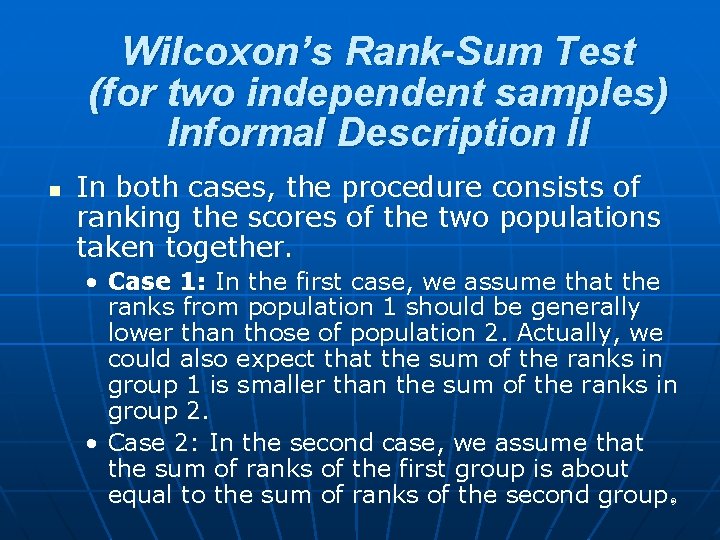
Wilcoxon’s Rank-Sum Test (for two independent samples) Informal Description II n In both cases, the procedure consists of ranking the scores of the two populations taken together. • Case 1: In the first case, we assume that the ranks from population 1 should be generally lower than those of population 2. Actually, we could also expect that the sum of the ranks in group 1 is smaller than the sum of the ranks in group 2. • Case 2: In the second case, we assume that the sum of ranks of the first group is about equal to the sum of ranks of the second group. 9

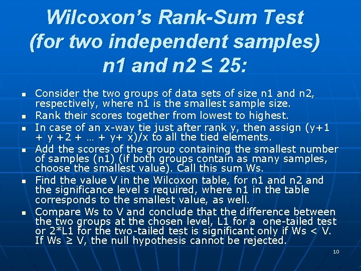
Wilcoxon’s Rank-Sum Test (for two independent samples) n 1 and n 2 ≤ 25: n n n Consider the two groups of data sets of size n 1 and n 2, respectively, where n 1 is the smallest sample size. Rank their scores together from lowest to highest. In case of an x-way tie just after rank y, then assign (y+1 + y +2 + … + y+ x)/x to all the tied elements. Add the scores of the group containing the smallest number of samples (n 1) (if both groups contain as many samples, choose the smallest value). Call this sum Ws. Find the value V in the Wilcoxon table, for n 1 and n 2 and the significance level s required, where n 1 in the table corresponds to the smallest value, as well. Compare Ws to V and conclude that the difference between the two groups at the chosen level, L 1 for a one-tailed test or 2*L 1 for the two-tailed test is significant only if Ws < V. If Ws ≥ V, the null hypothesis cannot be rejected. 10

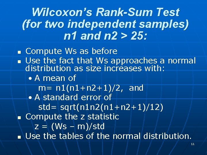
Wilcoxon’s Rank-Sum Test (for two independent samples) n 1 and n 2 > 25: n n Compute Ws as before Use the fact that Ws approaches a normal distribution as size increases with: • A mean of m= n 1(n 1+n 2+1)/2, and • A standard error of std= sqrt(n 1 n 2(n 1+n 2+1)/12) Compute the z statistic z = (Ws – m)/std Use the tables of the normal distribution. 11

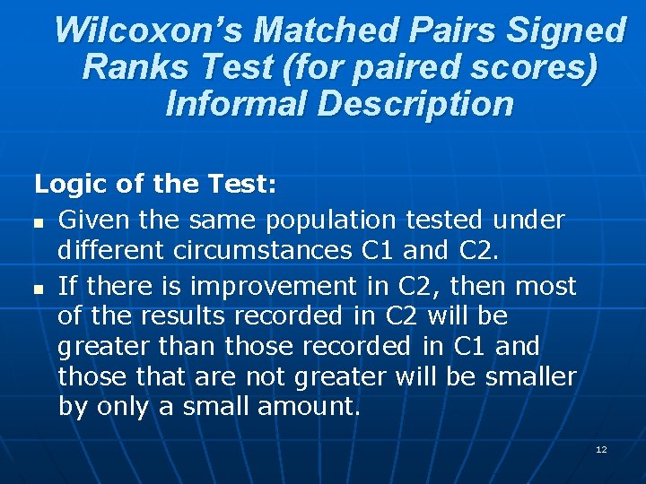
Wilcoxon’s Matched Pairs Signed Ranks Test (for paired scores) Informal Description Logic of the Test: n Given the same population tested under different circumstances C 1 and C 2. n If there is improvement in C 2, then most of the results recorded in C 2 will be greater than those recorded in C 1 and those that are not greater will be smaller by only a small amount. 12

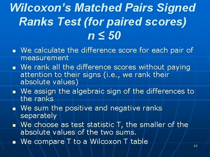
Wilcoxon’s Matched Pairs Signed Ranks Test (for paired scores) n ≤ 50 n n n We calculate the difference score for each pair of measurement We rank all the difference scores without paying attention to their signs (i. e. , we rank their absolute values) We assign the algebraic sign of the differences to the ranks We sum the positive and negative ranks separately We choose as test statistic T, the smaller of the absolute values of the two sums. We compare T to a Wilcoxon T table 13

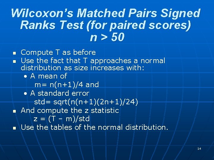
Wilcoxon’s Matched Pairs Signed Ranks Test (for paired scores) n > 50 n n Compute T as before Use the fact that T approaches a normal distribution as size increases with: • A mean of m= n(n+1)/4 and • A standard error std= sqrt(n(n+1)(2 n+1)/24) And compute the z statistic z = (T – m)/std Use the tables of the normal distribution. 14

Power Analysis 15

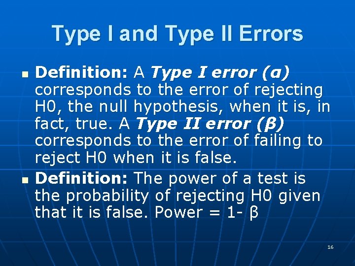
Type I and Type II Errors n n Definition: A Type I error (α) corresponds to the error of rejecting H 0, the null hypothesis, when it is, in fact, true. A Type II error (β) corresponds to the error of failing to reject H 0 when it is false. Definition: The power of a test is the probability of rejecting H 0 given that it is false. Power = 1 - β 16

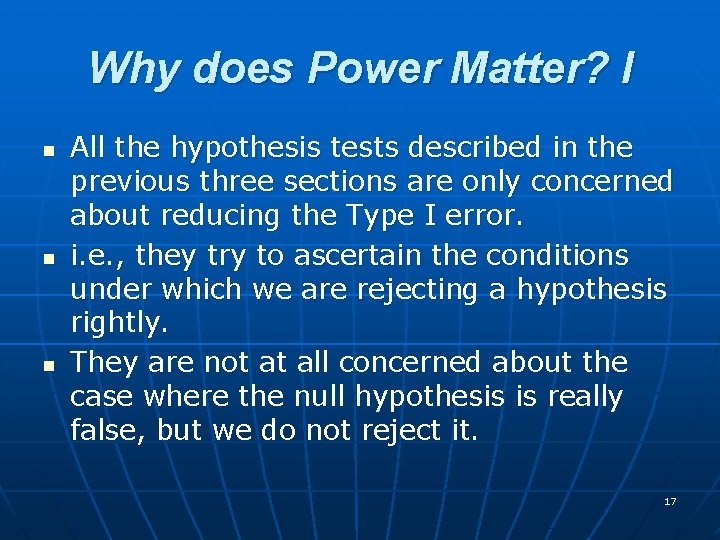
Why does Power Matter? I n n n All the hypothesis tests described in the previous three sections are only concerned about reducing the Type I error. i. e. , they try to ascertain the conditions under which we are rejecting a hypothesis rightly. They are not at all concerned about the case where the null hypothesis is really false, but we do not reject it. 17

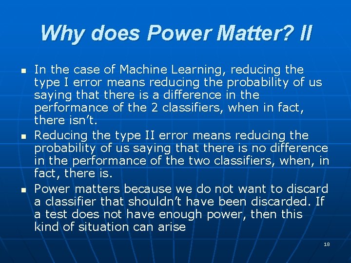
Why does Power Matter? II n n n In the case of Machine Learning, reducing the type I error means reducing the probability of us saying that there is a difference in the performance of the 2 classifiers, when in fact, there isn’t. Reducing the type II error means reducing the probability of us saying that there is no difference in the performance of the two classifiers, when, in fact, there is. Power matters because we do not want to discard a classifier that shouldn’t have been discarded. If a test does not have enough power, then this kind of situation can arise 18

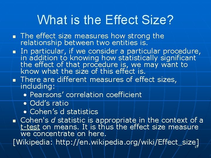
What is the Effect Size? The effect size measures how strong the relationship between two entities is. n In particular, if we consider a particular procedure, in addition to knowing how statistically significant the effect of that procedure is, we may want to know what the size of this effect is. n There are different measures of effect sizes, including: • Pearsons’ correlation coefficient • Odd’s ratio • Cohen’s d statistics n Cohen's d statistic is appropriate in the context of a t-test on means. It is thus the effect size measure we concentrate on here. [Wikipedia: http: //en. wikipedia. org/wiki/Effect_size 19] n

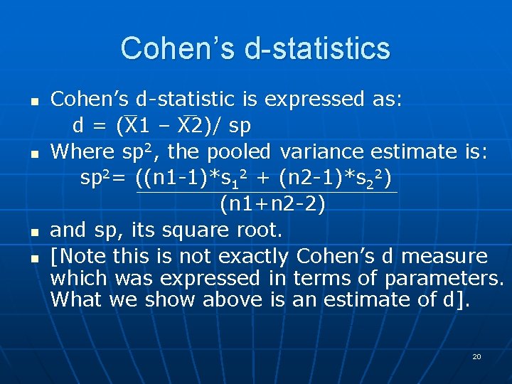
Cohen’s d-statistics n n Cohen’s d-statistic is expressed as: d = (X 1 – X 2)/ sp Where sp 2, the pooled variance estimate is: sp 2= ((n 1 -1)*s 12 + (n 2 -1)*s 22) (n 1+n 2 -2) and sp, its square root. [Note this is not exactly Cohen’s d measure which was expressed in terms of parameters. What we show above is an estimate of d]. 20

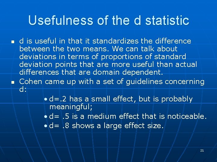
Usefulness of the d statistic n n d is useful in that it standardizes the difference between the two means. We can talk about deviations in terms of proportions of standard deviation points that are more useful than actual differences that are domain dependent. Cohen came up with a set of guidelines concerning d: • d=. 2 has a small effect, but is probably meaningful; • d=. 5 is a medium effect that is noticeable. • d=. 8 shows a large effect size. 21

Statistical Tests for Comparing Multiple Classifiers 22

What is the Analysis of Variance (ANOVA)? n n n The analysis of variance is similar to the t-test in that it deals with differences between sample means. However, unlike the t-test that is restricted to the difference between two means, ANOVA allows us to assess whether the differences observed between any number of means are statistically significant. In addition, ANOVA allows us to deal with more than one independent variable. For example, we could choose, as two independent variables, 1) the learning algorithm and 2) the domain to which the learning algorithm is applied. 23

Why is ANOVA useful? n n n One may wonder why ANOVA is useful in the context of classifier evaluation. Very simply, if we want to answer the following common question : "How do various classifiers fare on different data sets? ", then we have 2 independent variables: the learning algorithm and the domain, and a lot of results. ANOVA makes it easy to tell whether the difference observed are indeed significant. 24

Variations on the ANOVA Theme n There are different implementations of ANOVA: • One-way ANOVA is a linear model trying to assess if the difference in the performance measures of classifiers over different datasets is statistically significant, but does not distinguish between the performance measures’ variability within-datasets and the performance measure variability between-datasets. • Two-way/Multi-way ANOVA can deal with more than one independent variable. For instance, two performance measures over different classifiers over various datasets. n Then there are other related tests as well: 25 • Friedman’s test, Post-hoc tests, Tukey Test, etc…

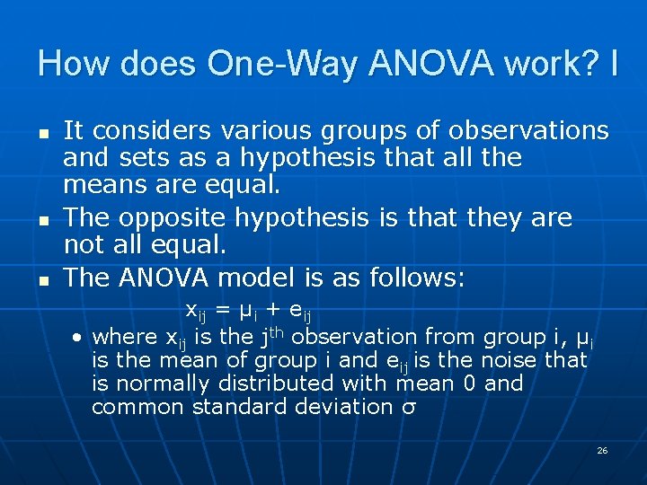
How does One-Way ANOVA work? I n n n It considers various groups of observations and sets as a hypothesis that all the means are equal. The opposite hypothesis is that they are not all equal. The ANOVA model is as follows: xij = μi + eij • where xij is the jth observation from group i, μi is the mean of group i and eij is the noise that is normally distributed with mean 0 and common standard deviation σ 26

How does One-Way ANOVA work? II n ANOVA monitors three different kinds of variation in the data: • Within-group variation • Between-group variation • Total variation = within-group variation + between-group variation n Each of the above variations are represented by sums of squares (SS) of the variations. The statistics of interest in ANOVA is F, where F = Between-group variation Within-group variation Larger F’s demonstrate greater statistical significance than smaller ones. Like for z and t, there are tables of significance levels associated with the F-ratio. 27

How does One-Way ANOVA work? III n n The goal of ANOVA is to find out whether or not the differences in means between different groups are statistically significant. To do so, ANOVA partitions the total variance into variance caused by random error (the within group SS) and variance caused by actual differences between means (the between-group SS). If the null hypothesis holds, then the within-group SS should be about the same as the betweengroups SS. We can compare these two SS using the F test, which checks whether the ratio of the two SSs is significantly greater than 1. 28

What is Multi-Way ANOVA? n n n In One-Way ANOVA, we simply considered several groups. For example this could correspond the comparing the performance of 10 different classifiers on one domain. How about the case where we compare the performance of these same 10 different classifiers on 5 domains? Two-Way ANOVA can help with that If we were to use an additional dimension such as the consideration of 6 different (but matched) threshold levels (as in AUC) for each classifier on the same 5 domains, then Three-way ANOVA could be used, and so on… 29

How Does Multi-Way ANOVA work? n In our example, the difference between One-Way ANOVA and Two-Way ANOVA can be illustrated as follows: • in One-Way ANOVA, we would calculate the within-group SS by collapsing the results obtained on all the data sets together within each classifier results. • In Two-Way ANOVA, with would calculate all the withinclassifier, within-domain variances separately and group the results together. • As a result, the spooled within-group SS of two-way ANOVA would be smaller than the spooled within-group SS of one-way ANOVA. n Multi-way ANOVA is thus a more statistically powerful test than One-way ANOVA since we need fewer observations to find significant effects. 30