CSI 5388 Error Estimation ReSampling Approaches 1 Error

- Slides: 24

CSI 5388 Error Estimation: Re-Sampling Approaches 1

Error Estimation n Error estimation is concerned with establishing whether the results we have obtained on a particular experiment are representative of the truth or whether they are meaningless. Traditionally, error estimation was performed using the classical parametric (and sometimes, non-parametric) tests discussed in Lecture 5. More recently, however, new tests have emerged for error estimation, based on re-sampling methods, that have the advantage of not making distributional assumptions the way parametric tests do. The tradeoff, though, is that such tests require high computational power. 2

Traditional Statistical Methods versus Resampling Methods n n n Classical parametric tests compare observed statistics to theoretical sampling distributions. Resampling makes statistical inferences based upon repeated sampling within the sample. Resampling methods stem from Monte Carlo simulations, but differ from them in that they are based upon some real data; Monte Carlo simulations, on the other hand, could be based on completely hypothetical data. 3

Error Estimation through Resampling Techniques in Machine Learning n n Error estimation through re-sampling techniques is concerned with finding the best way to utilize the available data to assess the quality of our algorithms. In other words, we want to make sure that our classifiers are tested on a variety of instances, within our sample, presenting different types of properties, so that we don't mistaken good performance on one type of instances as good performance across the entire domain. 4

Re-Sampling Approaches n We will be considering three different kinds of sampling approaches, with some of their variations in each case: • • n Cross-validation Jackknife (Leave-one-out) Bootstrapping Randomization The following discussion is based on • Yu, Chong Ho (2003): Resampling methods: concepts, applications and justification. Practical Assessment, Research & Evaluation, 8(19). • http: //www. uvm. edu/~dhowell/Stat. Pages/Resampling/Resamp ling. html, 5 • [Weiss & Kulikowski, 1991, Chapter 2]

Cross-Validation n A sample is randomly divided into two or more subsets and test results are validated by comparing across subsamples. The purpose of cross-validation is to find out whether the result is replicable or whether it is just a matter of random fluctuations. If the sample size is small, there is a chance that the results obtained are just artifacts of the sub-sample. In such cases, the jackknife procedure is preferred. 6

Jackknife n n n In the Jackknife or Leave-One-Out approach, rather than splitting the data set into several subsamples, all but one sample is used for training and the testing is done on the remaining sample. This procedure is repeated for all the samples in the data set. The procedure is preferable to cross-validation when the distribution is widely dispersed or in the presence of extreme scores in the data set. The estimate produced by the Jackknife approach is less biased, in the two cases mentioned above than cross-validation. 7

Bootstrapping and Randomization: Main Ideas n n n Bootstrapping makes the assumption that the sample is representative of the original distribution, and creates over a thousand bootstrapped samples by drawing, with replacement, from that pseudo-population. Randomization makes the same assumption, but, instead of drawing samples with replacement, it reorders (shuffles) the data systematically or randomly a thousand times or more. It calculates the appropriate test statistic on each reordering. Since shuffling the data amounts to sampling without replacement, the issue of replacement is one factor that differentiates the two approaches. 8

Bootsrapping n n One can understand the concept of bootstrapping by thinking of what can be done when not enough is known about the data. For example, let us assume that we don't know the standard error of the difference of medians. One solution consists of drawing many pairs of samples, calculating and recording, for each of these pairs of samples, the difference between the medians, and outputting the standard deviation of these differences in lieu of the standard error of the difference of medians. In other words, bootstrapping consists of using an empirical, brute-force solution when no analytical solution is available. Bootstrapping is also very useful in cases where the sample is too small for techniques such as crossvalidation or leave-one out to provide a good estimate, 9 due to the large variance a small sample will cause in such procedures.

The e 0 Bootstrap Estimator n n For the e 0 bootstrap, we create training and testing sets as follows: Given a data set consisting of n cases, we draw, with replacement, n samples from that set. The set of samples not included in the training set, thus created, forms the testing set. The error rate obtained on the test set represents one estimate of e 0. We repeat this procedure a number of times (between 50 and 200 times) and take the average of the results obtained for e 0. 10

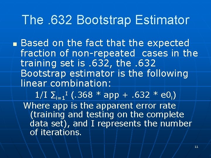
The. 632 Bootstrap Estimator n Based on the fact that the expected fraction of non-repeated cases in the training set is. 632, the. 632 Bootstrap estimator is the following linear combination: 1/I ∑i=1 I (. 368 * app +. 632 * e 0 i) Where app is the apparent error rate (training and testing on the complete data set), and I represents the number of iterations. 11

Bootstrapping versus Cross. Validation n n Both e 0 and. 632 B are low variance estimator. On the other hand, they are both more biased than cross-validation, which is nearly unbiased, but has high variance. • e 0 is pessimistically biased on moderately sized samples. Nonetheless, it gives good results in case of a high true error rate. • . 632 B becomes too optimistic as the sample size grows. However, it is a very good estimator on small data sets, especially if the true error rate is small. 12

Randomization Testing n n Randomization testing is closer in spirit to Classical parametric testing than Boostrapping. Bootstrapping proceeds to estimate the error directly. In contrast, randomization, testing like parametric testing, a null hypothesis gets tested. The null hypothesis of a randomization test, however, is quite different from that of a parametric tests (See next sets of slides) 13

Randomization versus Parametric Tests I n n n In randomization, we are not required to have random samples from one or two population(s). In randomization, we don’t think of the distribution from which the data comes. There is no assumption about normality or the like. The null hypothesis does not concern distributional parameters. Ø Instead, it is worded as a vague, but perhaps more easily interpretable, statement of the kind: “the treatment has no effect on the patient”, or perhaps, more precisely, as “the score that is associated with a participant is independent of the treatment that person received. ” 14

Randomization versus Parametric Tests II n n In randomization, we are not concerned with estimating or testing population parameters. Randomization testing does involve the computation of some sort of test statistic, but it does not compare that statistic to tabled distributions. The test statistics computed in randomization testing gets compared to the results obtained in repeating the same calculation over and over different randomizations of the data. Randomization testing is even more concerned about the random assignments of subjects to treatments (for example) than parametric tests. 15

Randomization: Basic Permutation Test • Decide on a metric to measure the effect in question. n For this example let’s use the t statistic (though several others are possible and equivalent, including the difference between the means) • Calculate that test statistic on the data (here denoted tobt). • Repeat the following N times, where N is a number greater than 1000 n n Shuffle the data Assign the first n 1 observations to the first condition, and the remaining n 2 observations to the secondition. Calculate the test statistic (here denoted ti*) for the reshuffled data. If ti* is greater than tobt increment a counter by 1. • Divide the value in the counter by N, to get the proportion of times the t on the randomized data exceeded the tobt on the data we actually obtained. • This is the probability of such an extreme result under the null. • Reject or retain the null hypothesis on the basis of this probability. 16

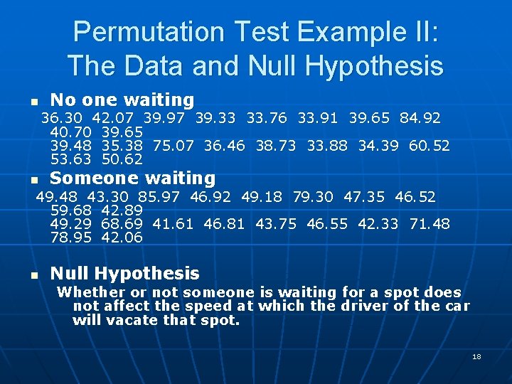
Permutation Test Example I: Two Independent Samples n n n Do drivers about to leave a parking space take more time than necessary if someone else is waiting for that spot? Ruback and Juieng, 1997 observed 200 drivers to answer this question. Howell reduced the data set to 20 samples under each condition (someone waiting or not), and modified the standard deviation appropriately to maintain the significant difference that they found. His data is reasonable in that it is positively skewed, because a driver can safely leave a space only so quickly, but, as we all know, he can sometimes take a very long time. Because the data are skewed, using a parametric t test may be problematic. So we will adopt a 17 randomization test.

Permutation Test Example II: The Data and Null Hypothesis n No one waiting 36. 30 42. 07 39. 97 39. 33 33. 76 33. 91 39. 65 84. 92 40. 70 39. 65 39. 48 35. 38 75. 07 36. 46 38. 73 33. 88 34. 39 60. 52 53. 63 50. 62 n Someone waiting 49. 48 43. 30 85. 97 46. 92 49. 18 79. 30 47. 35 46. 52 59. 68 42. 89 49. 29 68. 69 41. 61 46. 81 43. 75 46. 55 42. 33 71. 48 78. 95 42. 06 n Null Hypothesis Whether or not someone is waiting for a spot does not affect the speed at which the driver of the car will vacate that spot. 18

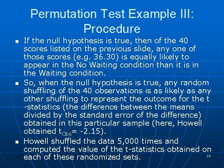
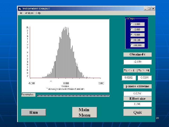
Permutation Test Example III: Procedure n n n If the null hypothesis is true, then of the 40 scores listed on the previous slide, any one of those scores (e. g. 36. 30) is equally likely to appear in the No Waiting condition than it is in the Waiting condition. So, when the null hypothesis is true, any random shuffling of the 40 observations is as likely as any other shuffling to represent the outcome for the t -statistics (the difference between the means divided by the standard error of the difference) obtained in this particular sample (here, Howell obtained t. Obs= -2. 15). Howell shuffled the data 5, 000 times and computed the value of the t-statistics obtained on 19 each of these randomized sets.

20

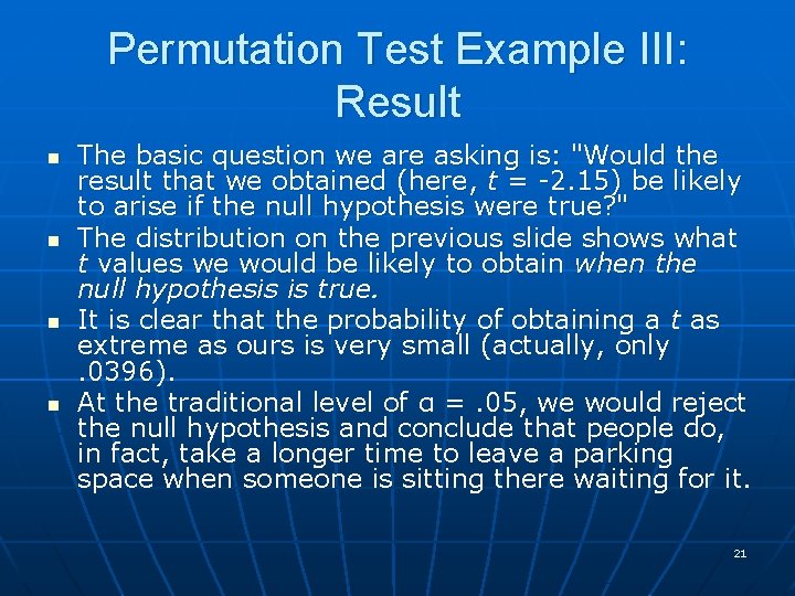
Permutation Test Example III: Result n n The basic question we are asking is: "Would the result that we obtained (here, t = -2. 15) be likely to arise if the null hypothesis were true? " The distribution on the previous slide shows what t values we would be likely to obtain when the null hypothesis is true. It is clear that the probability of obtaining a t as extreme as ours is very small (actually, only . 0396). At the traditional level of α =. 05, we would reject the null hypothesis and conclude that people do, in fact, take a longer time to leave a parking space when someone is sitting there waiting for it. 21

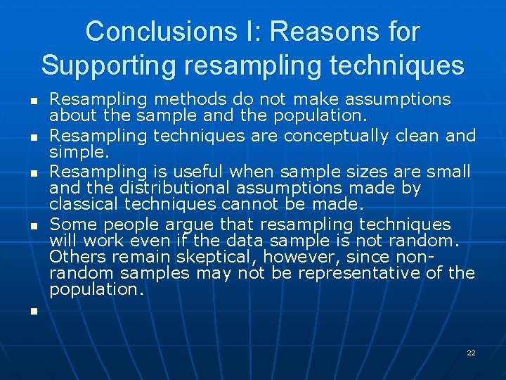
Conclusions I: Reasons for Supporting resampling techniques n n n Resampling methods do not make assumptions about the sample and the population. Resampling techniques are conceptually clean and simple. Resampling is useful when sample sizes are small and the distributional assumptions made by classical techniques cannot be made. Some people argue that resampling techniques will work even if the data sample is not random. Others remain skeptical, however, since nonrandom samples may not be representative of the population. 22

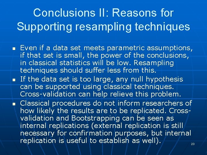
Conclusions II: Reasons for Supporting resampling techniques n n n Even if a data set meets parametric assumptions, if that set is small, the power of the conclusions, in classical statistics will be low. Resampling techniques should suffer less from this. If the data set is too large, any null hypothesis can be supported using classical techniques. Cross-validation can help relieve this problem. Classical procedures do not inform researchers of how likely the results are to be replicated. Crossvalidation and Bootstrapping can be seen as internal replications (external replication is still necessary for confirmation purposes, but internal replication is useful to establish as well). 23

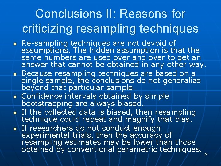
Conclusions II: Reasons for criticizing resampling techniques n n n Re-sampling techniques are not devoid of assumptions. The hidden assumption is that the same numbers are used over and over to get an answer that cannot be obtained in any other way. Because resampling techniques are based on a single sample, the conclusions do not generalize beyond that particular sample. Confidence intervals obtained by simple bootstrapping are always biased. If the collected data is biased, then resampling technique could repeat and magnify that bias. If researchers do not conduct enough experimental trials, then the accuracy of resampling estimates may be lower than those obtained by conventional parametric techniques. 24