CSE 881 Data Mining Lecture 22 Anomaly Detection

CSE 881: Data Mining Lecture 22: Anomaly Detection 1

Anomaly/Outlier Detection l What are anomalies/outliers? – Data points whose characteristics are considerably different than the remainder of the data l Applications: – – Credit card fraud detection telecommunication fraud detection network intrusion detection fault detection 2

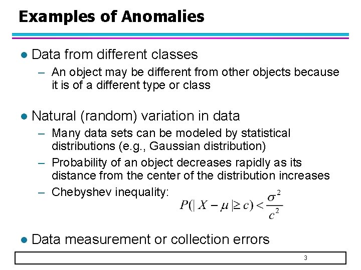
Examples of Anomalies l Data from different classes – An object may be different from other objects because it is of a different type or class l Natural (random) variation in data – Many data sets can be modeled by statistical distributions (e. g. , Gaussian distribution) – Probability of an object decreases rapidly as its distance from the center of the distribution increases – Chebyshev inequality: l Data measurement or collection errors 3

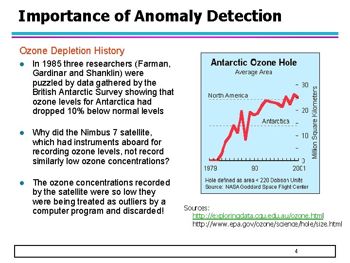
Importance of Anomaly Detection Ozone Depletion History l In 1985 three researchers (Farman, Gardinar and Shanklin) were puzzled by data gathered by the British Antarctic Survey showing that ozone levels for Antarctica had dropped 10% below normal levels l Why did the Nimbus 7 satellite, which had instruments aboard for recording ozone levels, not record similarly low ozone concentrations? l The ozone concentrations recorded by the satellite were so low they were being treated as outliers by a computer program and discarded! Sources: http: //exploringdata. cqu. edu. au/ozone. html http: //www. epa. gov/ozone/science/hole/size. html 4

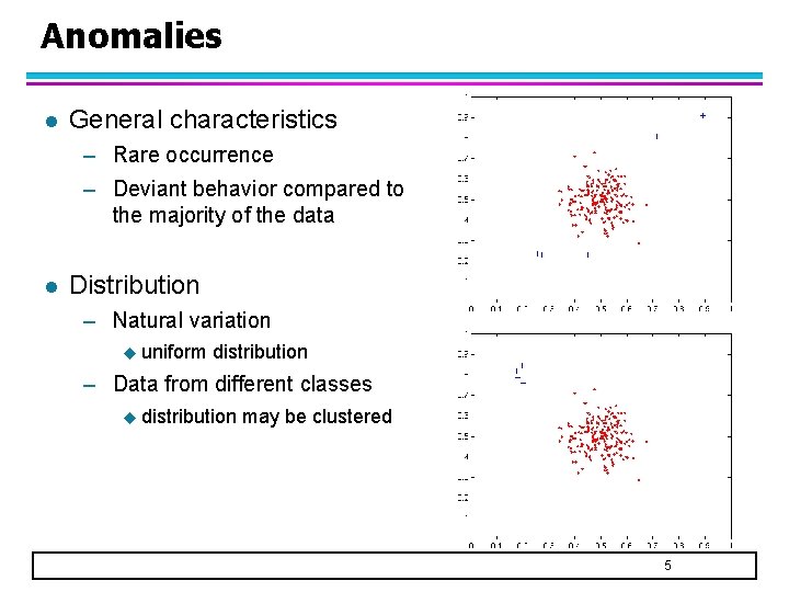
Anomalies l General characteristics – Rare occurrence – Deviant behavior compared to the majority of the data l Distribution – Natural variation u uniform distribution – Data from different classes u distribution may be clustered 5

Anomaly Detection l Challenges – Method is (mostly) unsupervised u Validation can be quite challenging (just like for clustering) – Small number of anomalies u Finding needle in a haystack 6

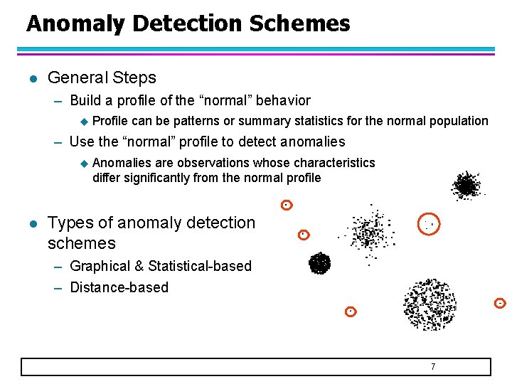
Anomaly Detection Schemes l General Steps – Build a profile of the “normal” behavior u Profile can be patterns or summary statistics for the normal population – Use the “normal” profile to detect anomalies u l Anomalies are observations whose characteristics differ significantly from the normal profile Types of anomaly detection schemes – Graphical & Statistical-based – Distance-based 7

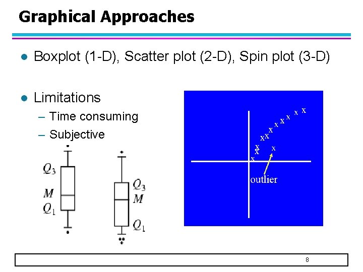
Graphical Approaches l Boxplot (1 -D), Scatter plot (2 -D), Spin plot (3 -D) l Limitations – Time consuming – Subjective 8

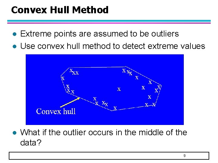
Convex Hull Method l l l Extreme points are assumed to be outliers Use convex hull method to detect extreme values What if the outlier occurs in the middle of the data? 9

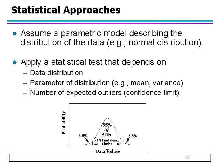
Statistical Approaches l Assume a parametric model describing the distribution of the data (e. g. , normal distribution) l Apply a statistical test that depends on – Data distribution – Parameter of distribution (e. g. , mean, variance) – Number of expected outliers (confidence limit) 10

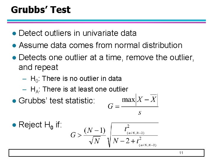
Grubbs’ Test Detect outliers in univariate data l Assume data comes from normal distribution l Detects one outlier at a time, remove the outlier, and repeat l – H 0: There is no outlier in data – HA: There is at least one outlier l Grubbs’ test statistic: l Reject H 0 if: 11

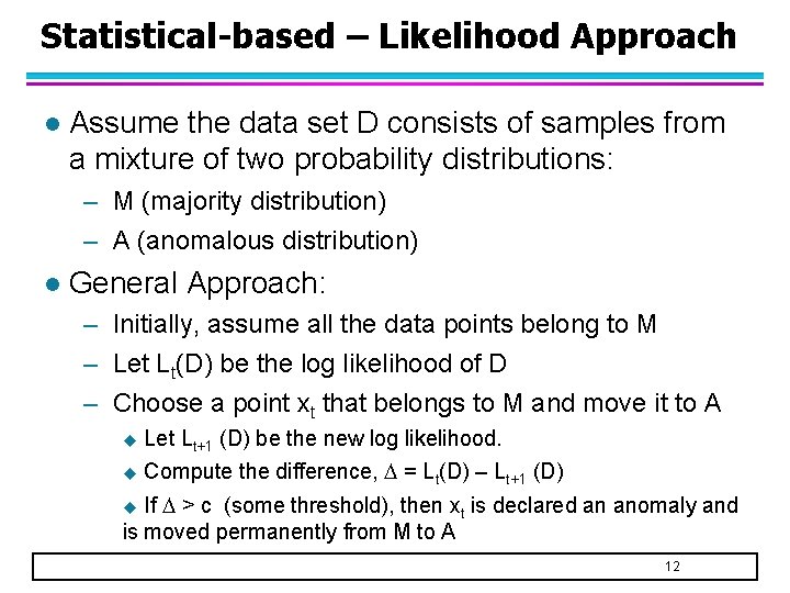
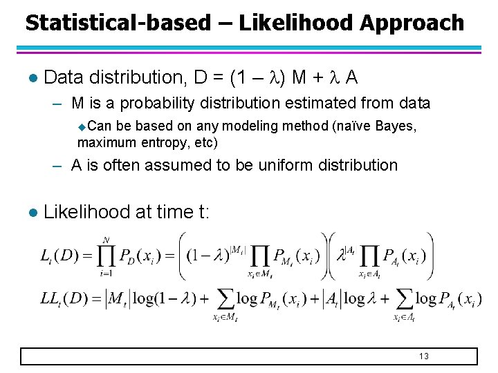
Statistical-based – Likelihood Approach l Assume the data set D consists of samples from a mixture of two probability distributions: – M (majority distribution) – A (anomalous distribution) l General Approach: – Initially, assume all the data points belong to M – Let Lt(D) be the log likelihood of D – Choose a point xt that belongs to M and move it to A u Let Lt+1 (D) be the new log likelihood. u Compute the difference, = Lt(D) – Lt+1 (D) If > c (some threshold), then xt is declared an anomaly and is moved permanently from M to A u 12

Statistical-based – Likelihood Approach l Data distribution, D = (1 – ) M + A – M is a probability distribution estimated from data u. Can be based on any modeling method (naïve Bayes, maximum entropy, etc) – A is often assumed to be uniform distribution l Likelihood at time t: 13

Limitations of Statistical Approaches l Most of the tests are for a single attribute l In many cases, the data distribution may not be known l For high dimensional data, it may be difficult to estimate the true distribution 14

Distance-based Approaches l Data is represented as a vector of features l Three approaches – Nearest-neighbor based – Density based – Clustering based 15

Nearest-Neighbor Based Approach l Approach: – Compute the distance between every pair of data points – There are various ways to define outliers: u Data points with fewer than p points within a neighborhood of radius D u Data points whose distance to the kth nearest neighbor is among the highest u Data points whose average distance to the k nearest neighbors is among the highest 16

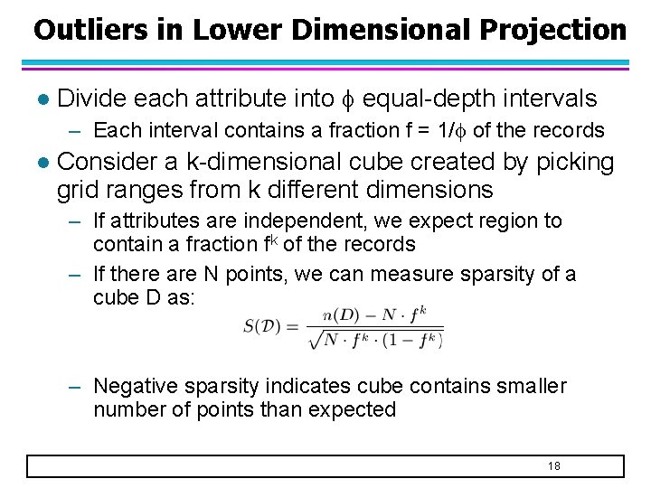
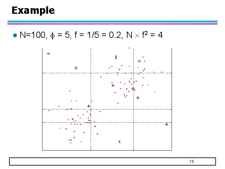
Outliers in Lower Dimensional Projection l Divide each attribute into equal-depth intervals – Each interval contains a fraction f = 1/ of the records l Consider a k-dimensional cube created by picking grid ranges from k different dimensions – If attributes are independent, we expect region to contain a fraction fk of the records – If there are N points, we can measure sparsity of a cube D as: – Negative sparsity indicates cube contains smaller number of points than expected 18

Example l N=100, = 5, f = 1/5 = 0. 2, N f 2 = 4 19

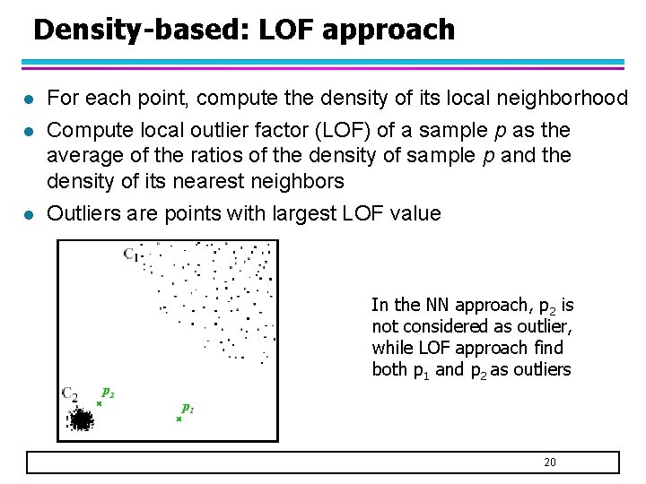
Density-based: LOF approach l l l For each point, compute the density of its local neighborhood Compute local outlier factor (LOF) of a sample p as the average of the ratios of the density of sample p and the density of its nearest neighbors Outliers are points with largest LOF value In the NN approach, p 2 is not considered as outlier, while LOF approach find both p 1 and p 2 as outliers p 2 p 1 20

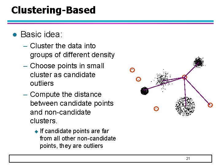
Clustering-Based l Basic idea: – Cluster the data into groups of different density – Choose points in small cluster as candidate outliers – Compute the distance between candidate points and non-candidate clusters. u If candidate points are far from all other non-candidate points, they are outliers 21

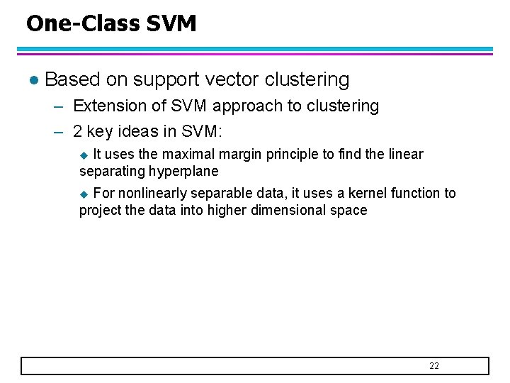
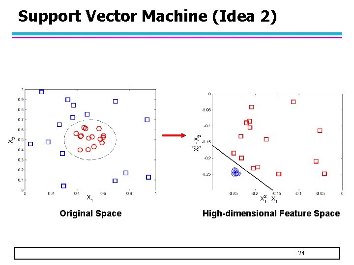
One-Class SVM l Based on support vector clustering – Extension of SVM approach to clustering – 2 key ideas in SVM: It uses the maximal margin principle to find the linear separating hyperplane u For nonlinearly separable data, it uses a kernel function to project the data into higher dimensional space u 22

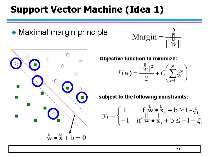
Support Vector Machine (Idea 1) l Maximal margin principle Objective function to minimize: subject to the following constraints: 23

Support Vector Machine (Idea 2) Original Space High-dimensional Feature Space 24

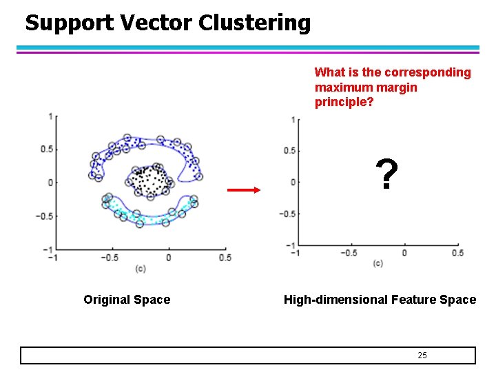
Support Vector Clustering What is the corresponding maximum margin principle? ? Original Space High-dimensional Feature Space 25

Support Vector Clustering l In SVM – Start with the simplest case first, then make the problem more complex – Simplest case: linearly separable data l Apply same idea to clustering – What is the simplest case? u All the points belong to a single cluster u The cluster is globular (spherical) 26

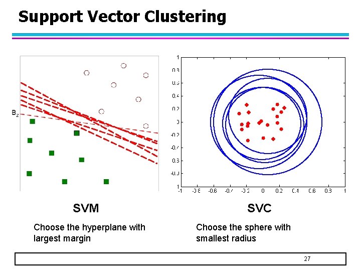
Support Vector Clustering SVM Choose the hyperplane with largest margin SVC Choose the sphere with smallest radius 27

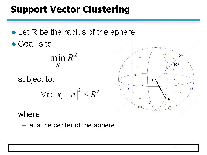
Support Vector Clustering Let R be the radius of the sphere l Goal is to: l subject to: a x where: – a is the center of the sphere 28

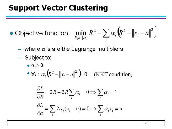
Support Vector Clustering l Objective function: – where I’s are the Lagrange multipliers – Subject to: u i 0 u 29

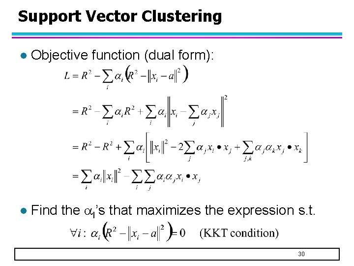
Support Vector Clustering l Objective function (dual form): l Find the I’s that maximizes the expression s. t. 30

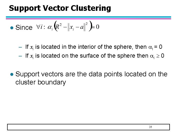
Support Vector Clustering l Since – If xi is located in the interior of the sphere, then i = 0 – If xi is located on the surface of the sphere then i 0 l Support vectors are the data points located on the cluster boundary 31

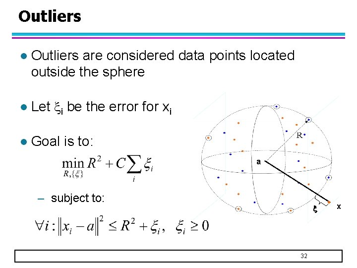
Outliers l Outliers are considered data points located outside the sphere l Let i be the error for xi l Goal is to: a – subject to: 32 x

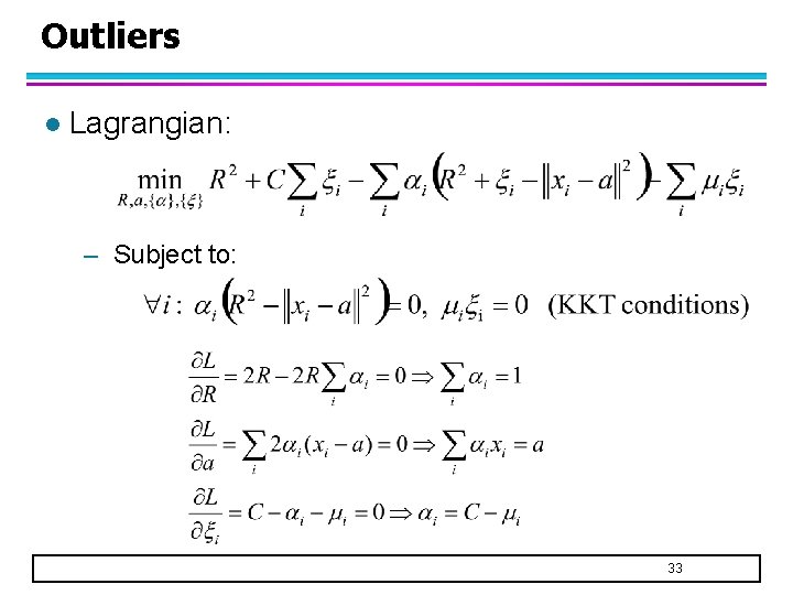
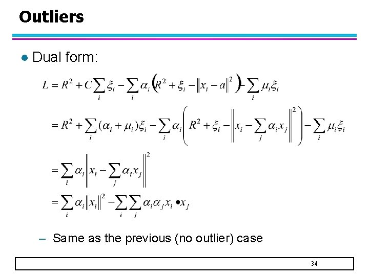
Outliers l Lagrangian: – Subject to: 33

Outliers l Dual form: – Same as the previous (no outlier) case 34

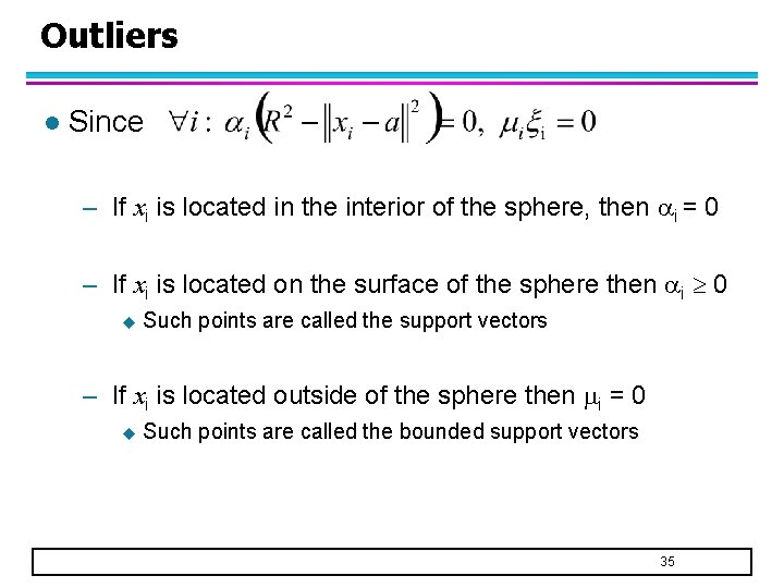
Outliers l Since – If xi is located in the interior of the sphere, then i = 0 – If xi is located on the surface of the sphere then i 0 u Such points are called the support vectors – If xi is located outside of the sphere then i = 0 u Such points are called the bounded support vectors 35

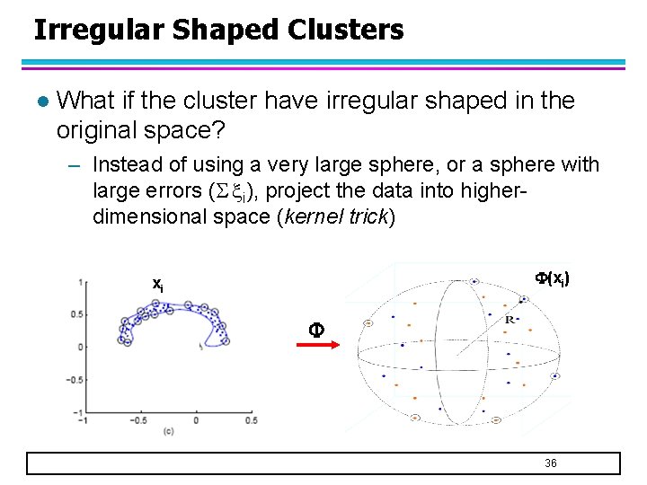
Irregular Shaped Clusters l What if the cluster have irregular shaped in the original space? – Instead of using a very large sphere, or a sphere with large errors ( i), project the data into higherdimensional space (kernel trick) (xi) xi 36

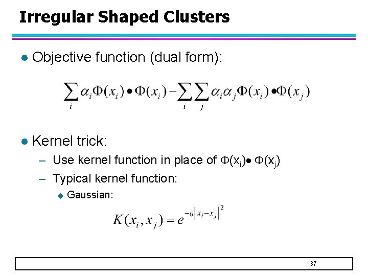
Irregular Shaped Clusters l Objective function (dual form): l Kernel trick: – Use kernel function in place of (xi) (xj) – Typical kernel function: u Gaussian: 37

References l Support Vector Clustering By Ben-Hur, Horn, Siegelmann, and Vapnik (Journal of Machine Learning Research, 2001) http: //citeseer. ist. psu. edu/hur 01 support. html l Cone Cluster Labeling for Support Vector Clustering By Lee and Daniels (in Proc. of SIAM Int’l Conf on Data Mining, 2006) http: //www. siam. org/meetings/sdm 06/proceedings/046 lees. pdf 38

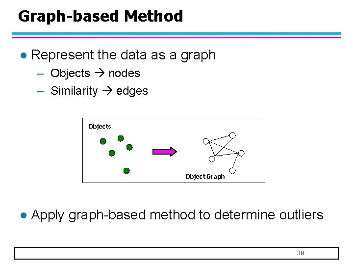
Graph-based Method l Represent the data as a graph – Objects nodes – Similarity edges Object Graph l Apply graph-based method to determine outliers 39

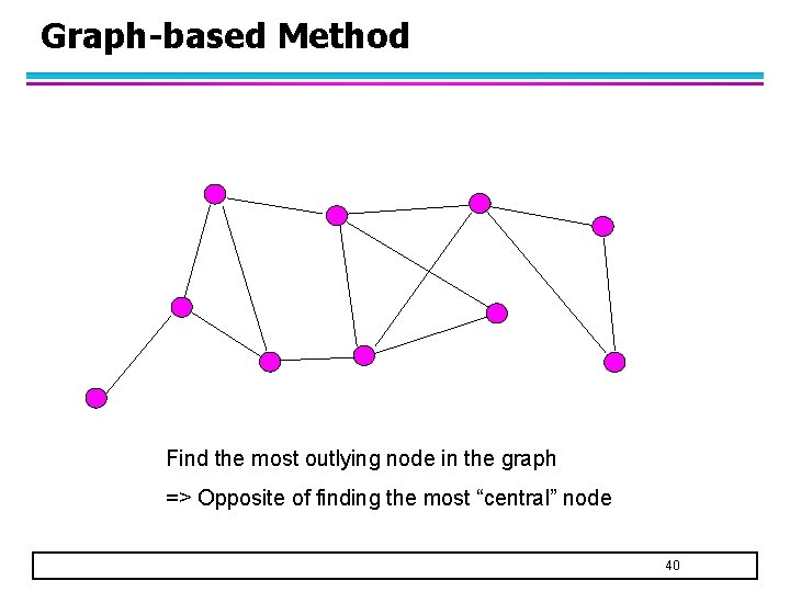
Graph-based Method Find the most outlying node in the graph => Opposite of finding the most “central” node 40

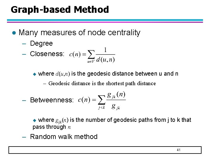
Graph-based Method l Many measures of node centrality – Degree – Closeness: u where d(u, n) is the geodesic distance between u and n – Geodesic distance is the shortest path distance – Betweenness: where gjk(n) is the number of geodesic paths from j to k that pass through n u – Random walk method 41

Random Walk Method l Random walk model – Randomly pick a starting node, s – Randomly choose a neighboring node linked to s. Set current node s to be the neighboring node. – Repeat step 2 l Compute the probability that you will reach a particular node in the graph – The higher the probability, the more “central” the node is. 42

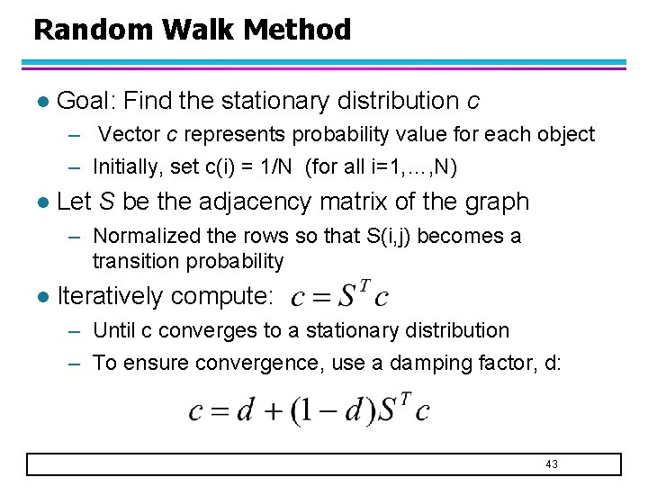
Random Walk Method l Goal: Find the stationary distribution c – Vector c represents probability value for each object – Initially, set c(i) = 1/N (for all i=1, …, N) l Let S be the adjacency matrix of the graph – Normalized the rows so that S(i, j) becomes a transition probability l Iteratively compute: – Until c converges to a stationary distribution – To ensure convergence, use a damping factor, d: 43

Random Walk Method l Applications – Web search (Page. Rank algorithm used by Google) – Text summarization – Keyword extraction 44

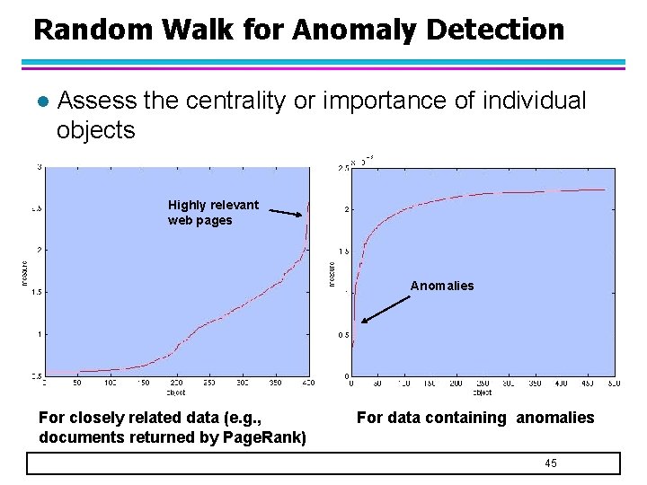
Random Walk for Anomaly Detection l Assess the centrality or importance of individual objects Highly relevant web pages Anomalies For closely related data (e. g. , documents returned by Page. Rank) For data containing anomalies 45

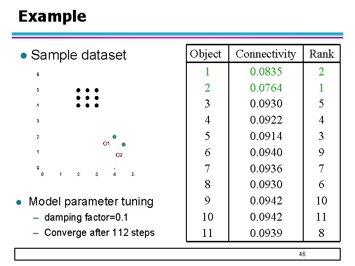
Example l l Sample dataset Model parameter tuning – damping factor=0. 1 – Converge after 112 steps Object 1 2 3 4 5 6 7 8 9 10 11 Connectivity 0. 0835 0. 0764 0. 0930 0. 0922 0. 0914 0. 0940 0. 0936 0. 0930 0. 0942 0. 0939 Rank 2 1 5 4 3 9 7 6 10 11 8 46