CSE 881 Data Mining Lecture 21 Graphbased Clustering

CSE 881: Data Mining Lecture 21: Graph-based Clustering 1

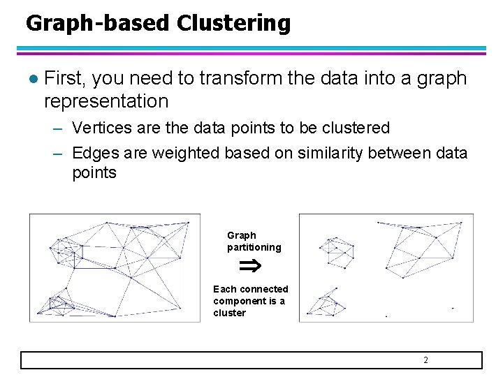
Graph-based Clustering l First, you need to transform the data into a graph representation – Vertices are the data points to be clustered – Edges are weighted based on similarity between data points Graph partitioning Each connected component is a cluster 2

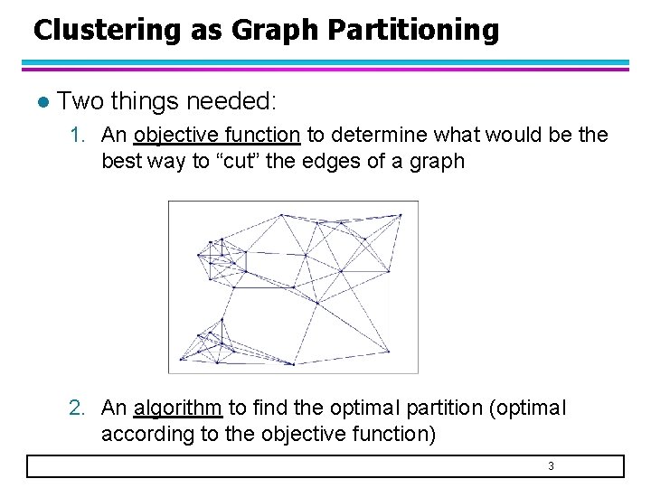
Clustering as Graph Partitioning l Two things needed: 1. An objective function to determine what would be the best way to “cut” the edges of a graph 2. An algorithm to find the optimal partition (optimal according to the objective function) 3

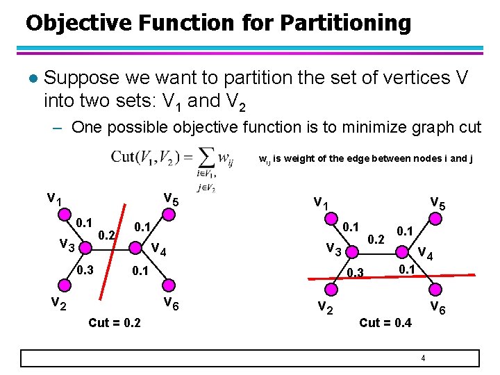
Objective Function for Partitioning l Suppose we want to partition the set of vertices V into two sets: V 1 and V 2 – One possible objective function is to minimize graph cut wij is weight of the edge between nodes i and j v 1 v 5 0. 1 v 3 0. 2 v 1 0. 1 v 4 v 3 0. 1 v 2 0. 3 v 6 Cut = 0. 2 v 5 v 2 0. 1 v 4 v 6 Cut = 0. 4 4

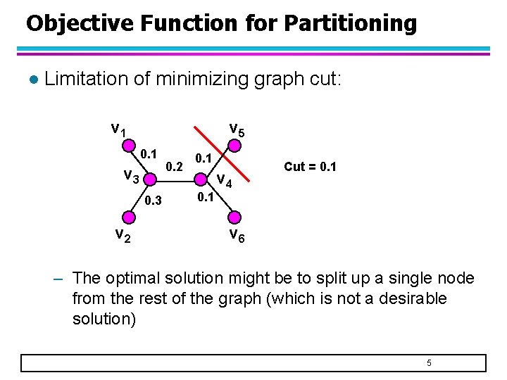
Objective Function for Partitioning l Limitation of minimizing graph cut: v 1 v 5 0. 1 v 3 0. 3 v 2 0. 1 v 4 Cut = 0. 1 v 6 – The optimal solution might be to split up a single node from the rest of the graph (which is not a desirable solution) 5

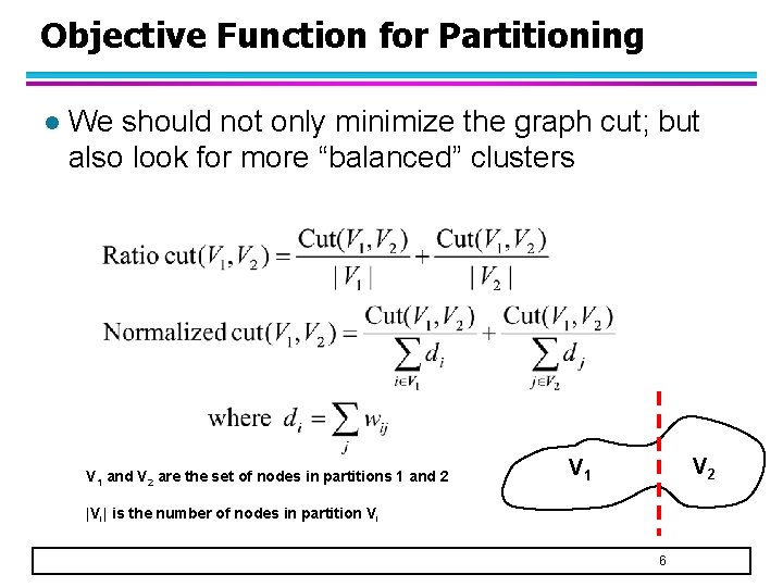
Objective Function for Partitioning l We should not only minimize the graph cut; but also look for more “balanced” clusters V 1 and V 2 are the set of nodes in partitions 1 and 2 V 1 |Vi| is the number of nodes in partition Vi 6

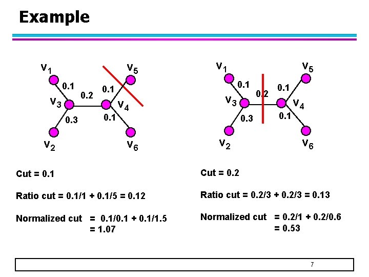
Example v 1 v 5 0. 1 v 3 0. 3 v 2 0. 2 v 5 0. 1 v 4 v 3 0. 3 v 6 v 2 0. 1 v 4 v 6 Cut = 0. 1 Cut = 0. 2 Ratio cut = 0. 1/1 + 0. 1/5 = 0. 12 Ratio cut = 0. 2/3 + 0. 2/3 = 0. 13 Normalized cut = 0. 1/0. 1 + 0. 1/1. 5 = 1. 07 Normalized cut = 0. 2/1 + 0. 2/0. 6 = 0. 53 7

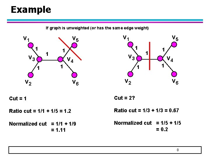
Example If graph is unweighted (or has the same edge weight) v 1 v 5 1 v 3 1 1 v 5 1 1 1 v 4 v 2 v 3 1 v 6 v 2 1 1 1 v 4 v 6 Cut = 1 Cut = 2? Ratio cut = 1/1 + 1/5 = 1. 2 Ratio cut = 1/3 + 1/3 = 0. 67 Normalized cut = 1/1 + 1/9 = 1. 11 Normalized cut = 1/5 + 1/5 = 0. 2 8

Algorithm for Graph Partitioning l Next, we need to design an algorithm that minimizes the objective function – We can use a heuristic (greedy) approach to do this u Example: METIS graph partitioning – But there are more elegant ways to optimize the function by using ideas from spectral graph theory This leads to a class of algorithms known as spectral clustering u 9

Spectral Clustering l Let’s examine the spectral properties of a graph – Spectral properties = eigenvalues/eigenvectors of the adjacency matrix representation of a graph l We then show the relationship between spectral properties of a graph and the graph partitioning problem 10

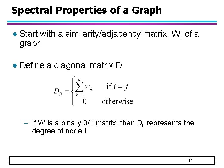
Spectral Properties of a Graph l Start with a similarity/adjacency matrix, W, of a graph l Define a diagonal matrix D – If W is a binary 0/1 matrix, then Dii represents the degree of node i 11

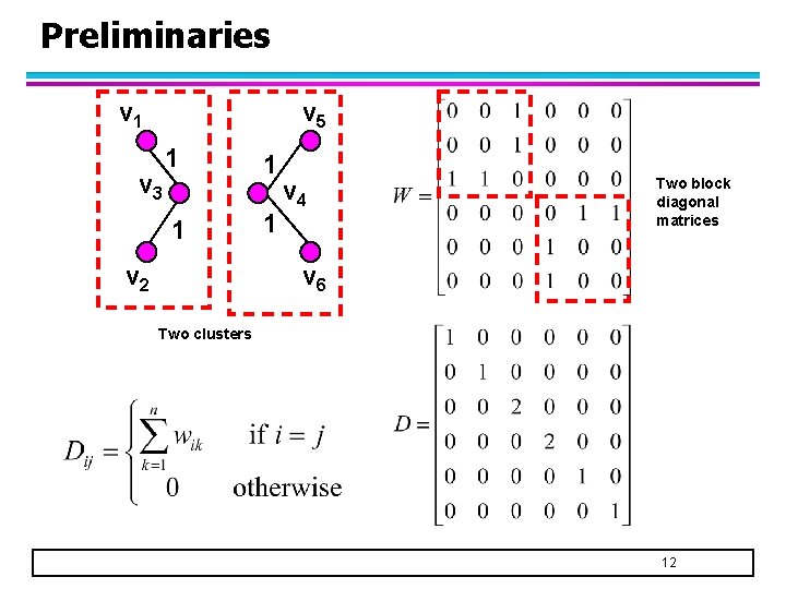
Preliminaries v 1 v 5 v 3 1 1 v 2 1 1 v 4 Two block diagonal matrices v 6 Two clusters 12

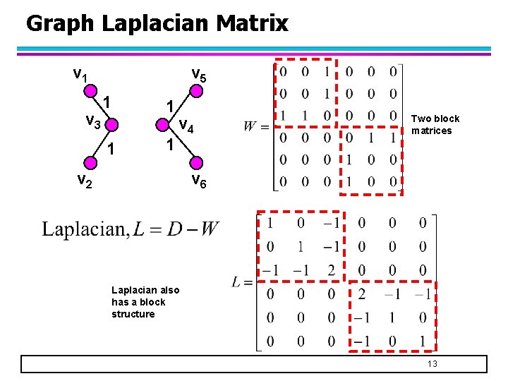
Graph Laplacian Matrix v 1 v 3 v 5 1 1 v 4 v 2 Two block matrices v 6 Laplacian also has a block structure 13

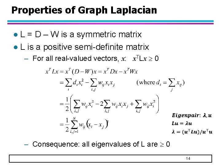
Properties of Graph Laplacian L = D – W is a symmetric matrix l L is a positive semi-definite matrix l – For all real-valued vectors, x: x. TLx 0 – Consequence: all eigenvalues of L are 0 14

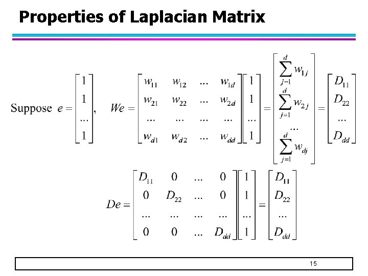
Properties of Laplacian Matrix 15

Properties of Laplacian Matrix l Since e [0. . 0]T, therefore = 0 – 0 is an eigenvalue of L with the corresponding eigenvector e = [1 1 1 1… 1]T – Furthermore, since L is positive semi-definite, 0 is the smallest eigenvalue of L 16

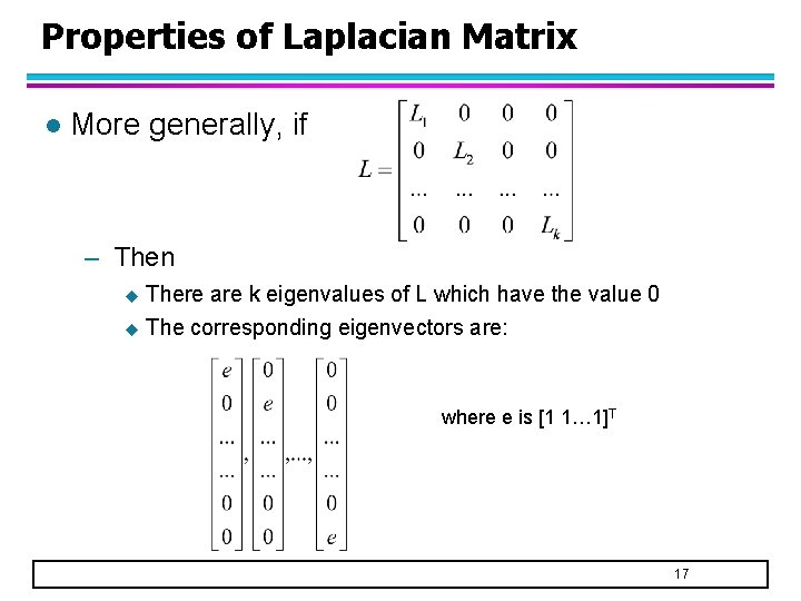
Properties of Laplacian Matrix l More generally, if – Then u There are k eigenvalues of L which have the value 0 u The corresponding eigenvectors are: where e is [1 1… 1]T 17

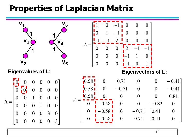
Properties of Laplacian Matrix v 1 v 3 v 5 1 1 v 2 Eigenvalues of L: 1 1 v 4 v 6 Eigenvectors of L: 18

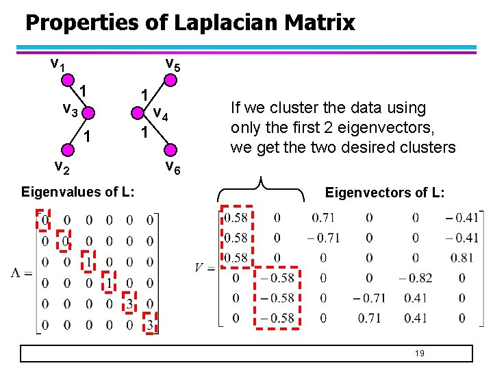
Properties of Laplacian Matrix v 1 v 3 v 5 1 1 v 2 Eigenvalues of L: 1 1 v 4 v 6 If we cluster the data using only the first 2 eigenvectors, we get the two desired clusters Eigenvectors of L: 19

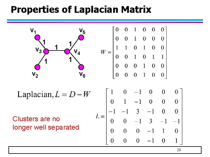
Properties of Laplacian Matrix v 1 v 3 v 5 1 1 v 2 1 1 1 v 4 v 6 Clusters are no longer well separated 20

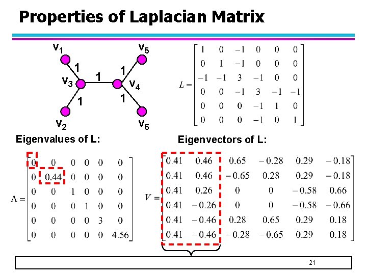
Properties of Laplacian Matrix v 1 v 3 v 5 1 1 1 v 2 Eigenvalues of L: 1 1 v 4 v 6 Eigenvectors of L: 21

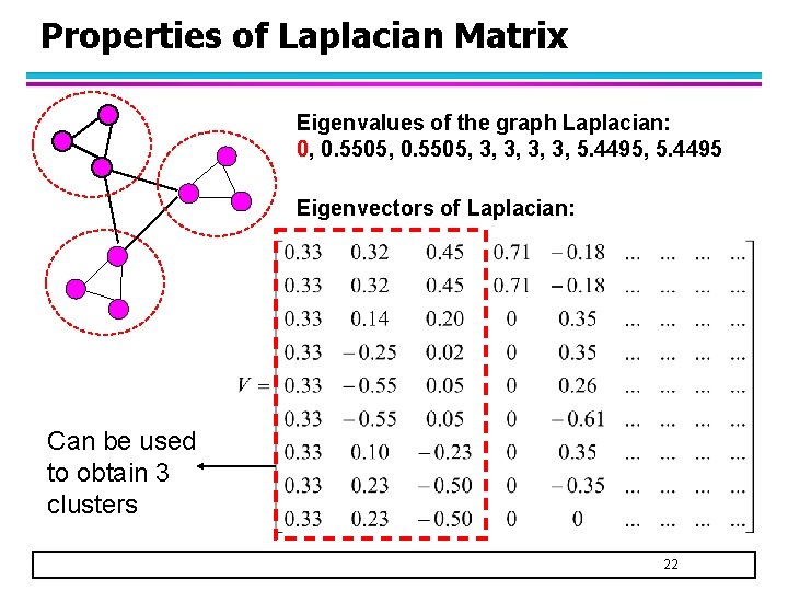
Properties of Laplacian Matrix Eigenvalues of the graph Laplacian: 0, 0. 5505, 3, 3, 5. 4495 Eigenvectors of Laplacian: Can be used to obtain 3 clusters 22

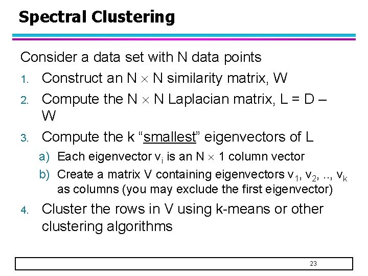
Spectral Clustering Consider a data set with N data points 1. Construct an N N similarity matrix, W 2. Compute the N N Laplacian matrix, L = D – W 3. Compute the k “smallest” eigenvectors of L a) Each eigenvector vi is an N 1 column vector b) Create a matrix V containing eigenvectors v 1, v 2, . . , vk as columns (you may exclude the first eigenvector) 4. Cluster the rows in V using k-means or other clustering algorithms 23

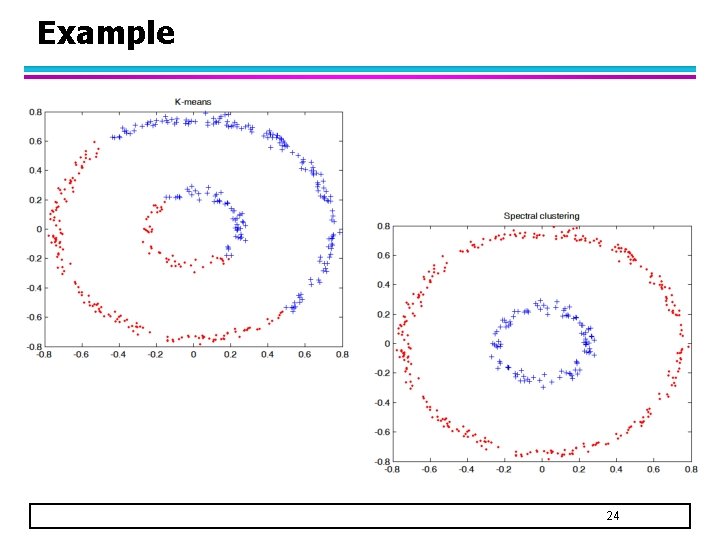
Example 24

Summary l Spectral properties of a graph (i. e. , eigenvalues and eigenvectors) contain information about clustering structure l To find k clusters, apply k-means or other algorithms to the first k eigenvectors of the graph Laplacian matrix 25

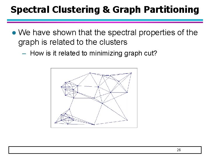
Spectral Clustering & Graph Partitioning l We have shown that the spectral properties of the graph is related to the clusters – How is it related to minimizing graph cut? 26

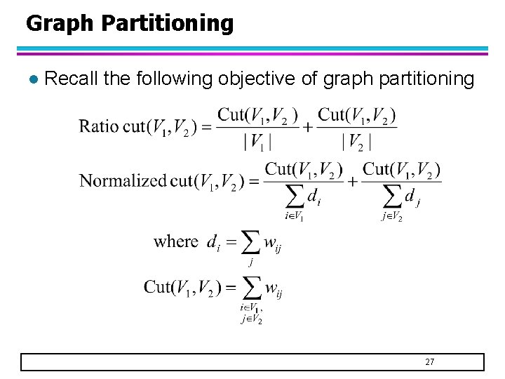
Graph Partitioning l Recall the following objective of graph partitioning 27

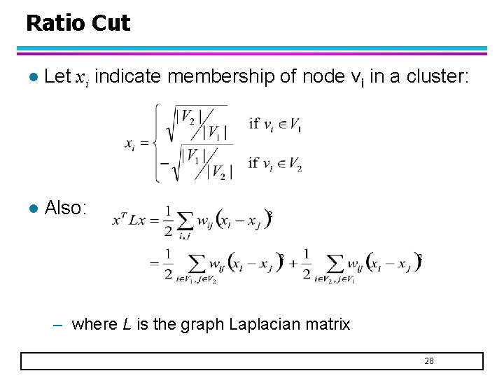
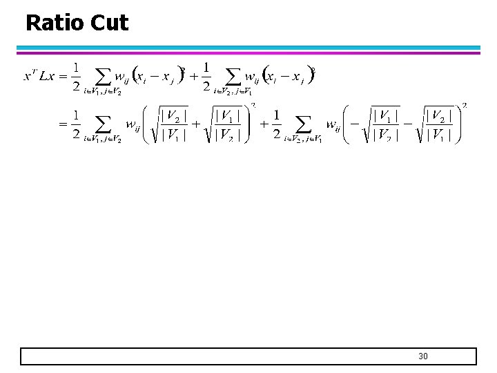
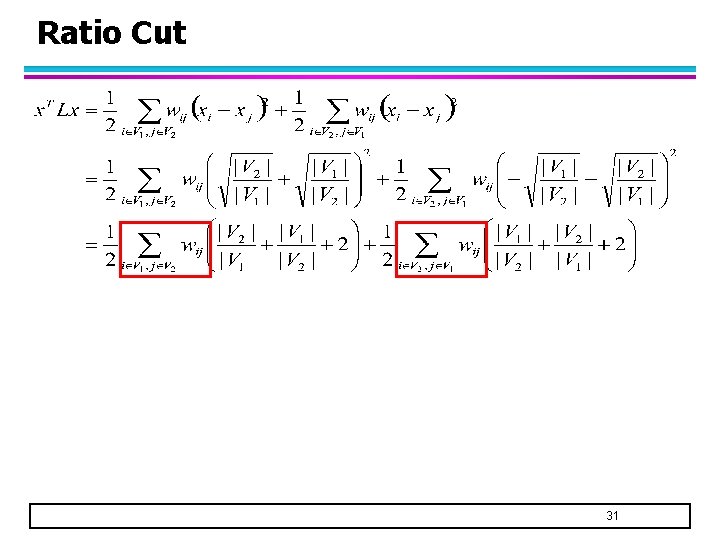
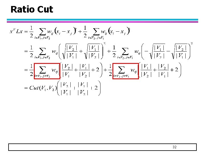
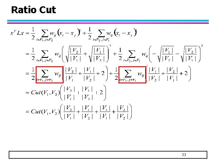
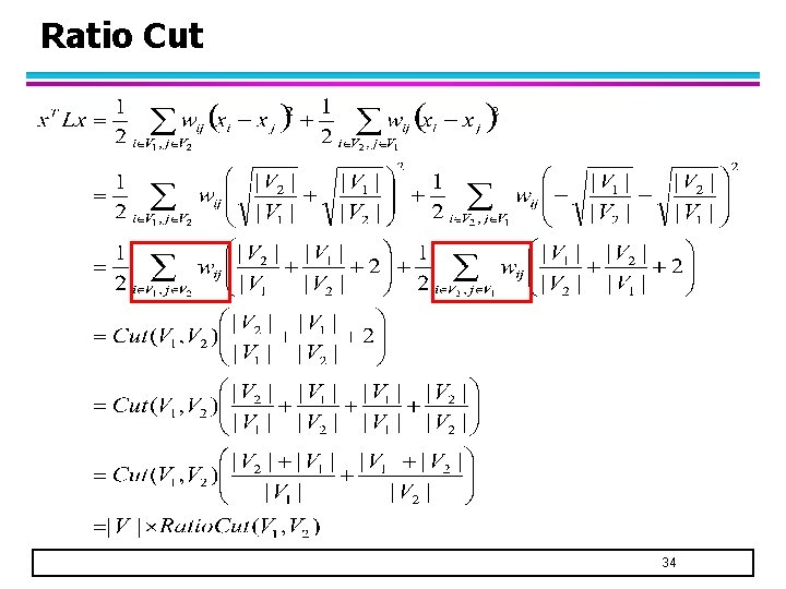
Ratio Cut l Let xi indicate membership of node vi in a cluster: l Also: – where L is the graph Laplacian matrix 28

Ratio Cut 29

Ratio Cut 30

Ratio Cut 31

Ratio Cut 32

Ratio Cut 33

Ratio Cut 34

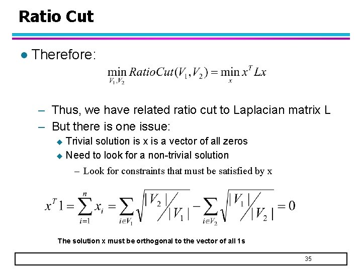
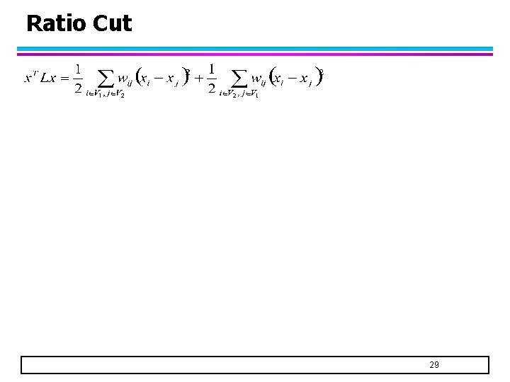
Ratio Cut l Therefore: – Thus, we have related ratio cut to Laplacian matrix L – But there is one issue: Trivial solution is x is a vector of all zeros u Need to look for a non-trivial solution u – Look for constraints that must be satisfied by x The solution x must be orthogonal to the vector of all 1 s 35

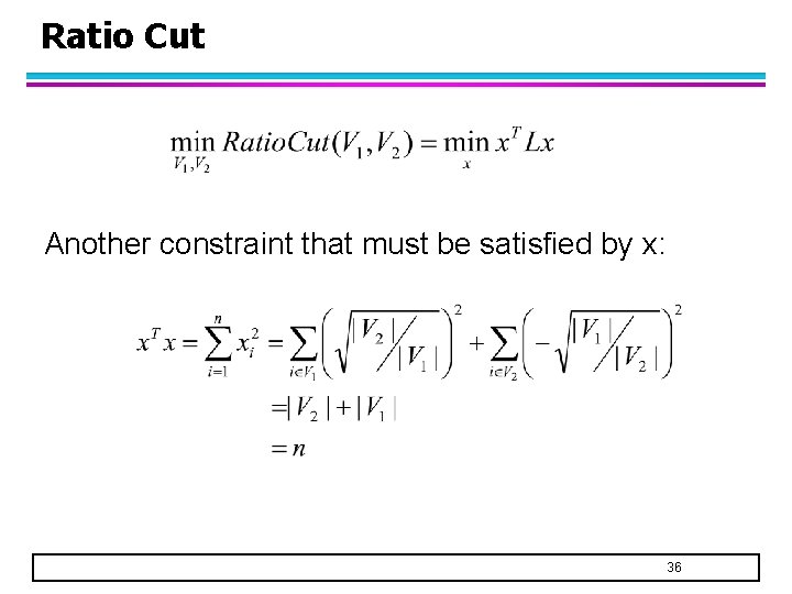
Ratio Cut Another constraint that must be satisfied by x: 36

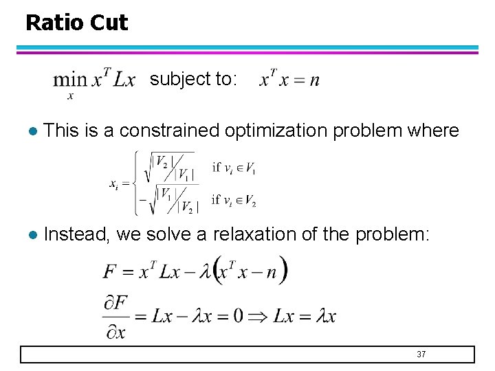
Ratio Cut subject to: l This is a constrained optimization problem where l Instead, we solve a relaxation of the problem: 37

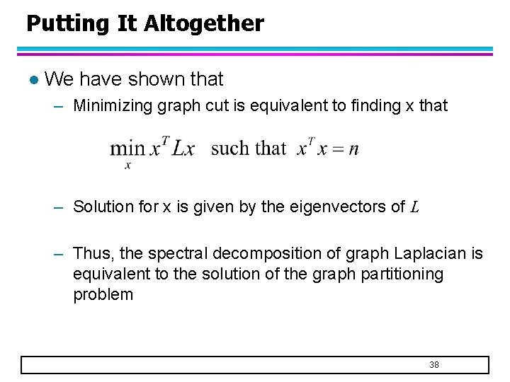
Putting It Altogether l We have shown that – Minimizing graph cut is equivalent to finding x that – Solution for x is given by the eigenvectors of L – Thus, the spectral decomposition of graph Laplacian is equivalent to the solution of the graph partitioning problem 38

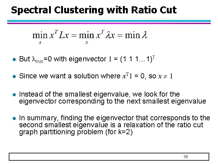
Spectral Clustering with Ratio Cut l But min=0 with eigenvector 1 = (1 1 1… 1)T l Since we want a solution where x. T 1 = 0, so x 1 l Instead of the smallest eigenvalue, we look for the eigenvector corresponding to the next smallest eigenvalue l In summary, finding the eigenvector that corresponds to the second smallest eigenvalue is a relaxation of the ratio cut graph partitioning problem (for k=2) 39