CSE 551 Computational Methods 20182019 Fall Chapter 7

CSE 551 Computational Methods 2018/2019 Fall Chapter 7 Systems of Linear Equations

Outline Naive Gaussian Elimination with Scaled Partial Pivoting Tridiagonal and Banded Systems Matix Factorizations

References • W. Cheney, D Kincaid, Numerical Mathematics and Computing, 6 ed, • Chapter 7 • Chapter 8

Naive Gaussian Elimination A Larger Numerical Example Algorithm Pseudocode Testing the Pseudocode Residual and Error Vectors

Naive Gaussian Elimination • fundamental problems in many scientific and engineering applications is to • solve an algebraic linear system Ax = b – – for the unknown vector x the coefficient matrix A and right-hand side vector b known • arise – various applications; – approximating nonlinear equations by linear equations – or differential equations by algebraic equations • • • cornerstone of many numerical methods the efficient and accurate solution of linear systems The system of linear algebraic equations Ax = b may or may not have a solution if it has a solution, it may or may not be unique.

• Gaussian elimination – standard method for solving the linear system • When the system has no solution – other approaches, e. g. , linear least squares • assume that: – the coefficient matrix A is n × n and – invertible (nonsingular) • pure mathematics - solution of Ax = b : x =A− 1 b – A− 1: inverse matrix. • most applications - solve the system directly for the unknown vector x

• many applications, daunting task: – to solve accurately extremely large systems - thousands or millions of unknowns • Some questions: – – – – How to store such large systems in the computer? Are computed answers correct? What is the precision of the computed results? Can the algorithm fail? How long will it take to compute answers? What is the asymptotic operation count of the algorithm? Will the algorithm be unstable for certain systems? Can instability be controlled by pivoting? (Permuting the order of the rows of the matrix is called pivoting. ) – Which strategy of pivoting should be used? – Whether the matrix is ill-conditioned? – whether the answers are accurate?

• Gaussian elimination transforms a linear system into an upper triangular form – easier to solve • process equivalent to finding the factorization – – A = LU L: unit lower triangular matrix U: upper triangular matrix This • useful solving many linear systems – the same coefficient matrix – different right-hand sides

• When A - special structure: – symmetric, positive definite, triangular, banded, block, or sparse • Gaussian elimination with partial pivoting – modified or rewritten specifically for th system.

• develop a good program for solving a system of n • linear equations in n unknowns: • In compact form:

A Larger Numerical Example • simplest form of Gaussian elimination - naive • not suitable for automatic computation – essential modifications • e. g. , naive Gaussian elimination:

first step • elimination procedure: • certain multiples of the first equation – – subtracted from the second, third, and fourth equations eliminate x 1 from these equations. to create 0’s as coefficients for each x 1 below the first 12, 3, − 6 stand • subtract 2 times the first equation from the second – multiplier: 12/6. • subtract 12 times the first equation from the third – multiplier: 3/6 • subtract − 1 times the first equation from the fourth.

• the first equation not altered pivot equation • Systems (2) and (3) are equivalent: – Any solution of (2) is also a solution of (3)

second step • ignore the first equation and the first column of coefficients • system of three equations with three unknowns same process repeated: – the top equation in the smaller system current pivot equation • subtracting 3 times the second equation from the third. – multiplier: − 12/(-4) • subtract − 1/2 times the second equation from the fourth

• final step: – subtracting 2 times the third equation from the fourth: • system is in upper triangular form • equivalent to System (2)

• • • completes first phase (forward elimination) The second phase (back substitution) solve System (5) for the unknowns starting at the bottom from the fourth equation: Putting x 4 = 1 in the third equation: • The solution:

Algorithm • • write System (1) in matrix-vector form ai j: n × n square array, or matrix unknowns xi right-hand side elements bi : n× 1 arrays, or vectors • or

• Operations between equations correspond to operations between rows in this notation • naive Gaussian elimination algorithm for the general system, – n equations and n unknowns • original data are overwritten

forward elimination phase • n − 1 principal steps • first step: first equation to produce n − 1 • zeros as coefficients for each x 1 in all other equations i, i >1 – subtracting appropriate multiples of the first equation from the others • first equation - first pivot equation • a 11 as the first pivot element

• remaining equations (2 i n): • ← : replacement – content of the memory location allocated to ai j replaced by ai j − (ai 1/a 1 1)a 1 j , and so on. • (ai 1/a 11) multipliers • new coefficient of x 1 in the ith equation: 0 • ai 1 − (ai 1/a 11)a 11 = 0.

• After the first step,

• not alter first equation • not alter coefficients x 1 – a multiplier times 0 subtracted from 0 is still 0 • ignore the first row and the first column • repeat the process on the smaller system. • With the second equation - pivot equation: – compute for each remaining equation (3 i n)

• prior to the kth step, the system: • • a wedge of 0 coefficients created first k equations processed - now fixed kth equation - pivot equation select multipliers - create 0’s coefficients xi below the akk coefficient.

• compute for each remaining equation – (k + 1 i n) • assume that all the divisors in this algorithm are nonzero

Pseudocode • • pseudocode forward elimination coefficient array: (ai j ) right-hand side of the system of equations: (bi ) solution computed: (xi )

• multiplier aik/akk not depend on j • moved outside the j loop • the new values in column k will be 0 -theoretically, when j = k:

• The location where the 0 created good place to store multiplie :

• At the beginning of the back substitution phase, • the linear system: • the ai j’s and bi’s not original ones from System (6) • altered by the elimination process

• The back substitution starts by solving the nth equation for xn: • using the (n − 1)th solve for xn− 1: • continue upward, recovering each xi:

pseudocode of back substitution

procedure Naive Gauss

• crucial computation: • a triply nested for-loop containing a replacement operation:

• expect all quantities to be infected with roundoff error • Such a roundoff error • in ak j multiplied by the factor (aik/akk) • large: pivot element |akk | small relative to |aik |. • conclude, tentatively, that – small pivot elements lead to – large multipliers and to worse roundoff errors.

Testing the Pseudocode • One way to test a procedure: – set up an artificial problem – solution is known beforehand • test problem - parameter – changed to vary the difficulty. • example: • Fixing n:

• coefficients all equal to 1 • try to recover known coefficients – values of p(t) at integers t = 1+i for i = 1, 2, . . . , n • coefficients: x 1, x 2, . . . , xn: • used formula sum of a geometric series on the right-hand side: • linear system

Example • write a pseudocode for a specific test case that solves the system of Equation (8) for various values of n. • Solution: use Naive Gauss • calling program: n = 4, 5, 6, 7, 8, 9, 10 • for testing

pseudocode

• run on a machine approximately seven decimal digits of accuracy • solution with complete precision until n reached 9, • then, the computed solution worthless – one component exhibited a relative error of 16, 120%!

• • The coefficient matrix for this linear system example of a well-known illconditioned matrix the Vandermonde matrix cannot be solved accurately - naive Gaussian elimination amazing the trouble happens so suddenly! n: 9 roundoff error - computing xi propagated and magnified throughout the back substitution phase • most computed values for xi worthless • Insert intermediate print statements • to see what is going on here. Res

Residual and Error Vectors • linear system Ax = b - true solution x • and a computed solution • define: • relationship between the error vector and the residual vector:

• using different computers solve the same linear system, Ax = b • algorithm and precision not known • two solutions xa and xb totally different! • How determine which, if either, computed solution is correct?

• check the solutions substituting them into the original system, • computing the residual vectors: ra = Axa − b and rb = Axb − b • computed solutions not exact • some roundoff errors • accept the solution with the smaller residual vector. • However, if we knew • the exact solution x, then we would just compare the computed solutions with the exact • solution, which is the same as computing the error vectors ea = x −xa and eb = x −xb • computed solution - smaller error vector • most assuredly be the better answer

• • exact solution not known accept the computed solution - smaller residual vector may not be the best computed solution original problem sensitive to roundoff errors illconditioned. the question: whether a computed solution to a linear system is a good solution is extremely difficult

Gaussian Elimination with Scaled Partial Pivoting Naive Gaussian Elimination Can Fail Partial Pivoting and Complete Partial Pivoting Gaussian Elimination with Scaled Partial Pivoting A Larger Numerical Example Pseudocode Long Operation Count Numerical Stability Scaling

Naive Gaussian Elimination Can Fail • naive Gaussian elimination algorith unsatisfactory: • the algorithm fails if a 11 = 0. • If fails for some values of the data • untrustworthy - values near the failing values: • ε small number different from 0

• naive algorithm works • after forward elimination: • back substitution: • ε− 1 large - computer – fixed word length • small ε, (2 − ε− 1), (1 − ε− 1) computed as −ε− 1

• 8 -digit decimal machine with a 16 -digit accumulator, when ε =10− 9 • ε− 1 = 109 • subtract -interpret the number: • ε− 1− 2 computed: 0. 099998 00000 0 × 1010 rounded to 0. 10000 000× 1010 = ε− 1

• for values of ε sufficiently close to 0 • computer calculates x 2: 1 x 1: 0 • correct solution: • relative error x 1: 100%

• naive Gaussian elimination algorithm works well on Systems (1) and (2) • if the equations are first permuted: x 2 = 1, x 1 = 2 - x 2=1

• second systems: • forward elimination and back substitution: • • not to rearrange the equations select a different pivot row difficulty in (2): not ε small but small relative to other coefficients in the same row

• To verify: • (4) equivalent to (2) • The naive Gaussian elimination algorithm fails • triangular system • back substitution - erroneous result

• resolved interchanging the two equations in (4): • naive Gaussian elimination algorithm: • correct solution

Partial Pivoting and Complete Partial Pivoting • Gaussian elimination with partial pivoting selects the pivot row to be the one with the maximum pivot entry in absolute value from those in the leading column of the reduced submatrix • Two rows are interchanged to move the designated row into the pivot row position. • Gaussian elimination with complete pivoting selects the pivot entry as the maximum pivot entry from all entries in the submatrix • (This complicates things because some of the unknowns are rearranged. ) • Two rows and two columns are interchanged to accomplish this. • In practice, partial pivoting is almost as good as full pivoting and involves significantly less work

• Simply picking the largest number in magnitude as is done in partial pivoting may work well, but here row scaling does not play a role—the relative sizes of entries in a row are not considered. • Systems with equations having coefficients of disparate sizes may cause difficulties and should be viewed with suspicion • Sometimes a scaling strategy may ameliorate these problems • present Gaussian elimination with scaled partial pivoting, and the pseudocode contains an implicit pivoting scheme.

• Gaussian elimination with the simple partial pivoting strategy may incorrect solution: • c - can - very large values • first row - pivot row: – the larger number in the first column • multiplier: 1/2, one step in the row reduction process:

• computer limited word length 1 − c ≈ −c, 2 − c ≈ −c. • so: • y = 1, x = 0 • correct solution: x = y = 1

• Gaussian elimination with scaled partial pivoting selects second row - pivot row • scaling constants: (2 c, 1) • larger of the two ratios - selecting the pivot row: • {2/(2 c), 1} - second one • multiplier: 2, • one step in the row reduction process:

• computer of limited word length 2 c − 2 ≈ 2 c, 2 c − 4 ≈ 2 c • compute: • obtain the correct solution: • y = 1, x = 1

Gaussian Elimination with Scaled Partial Pivoting • the order treat the equations significantly affects the accuracy of the elimination algorithm • naive Gaussian elimination algorithm • order equations - pivot equations natural order {1, 2, . . . , n} • equation: n not used as an operating equation: • no multiples of it subtracted from other equations

• strategy - selecting new pivots • best approach - complete pivoting, • searches all entries in the submatrices for the largest entry in absolute value – interchanges rows and columns to move it into the pivot position – great amount of searching and data movement. • searching the first column in the submatrix at each stage (avoiding small or zero pivots)

• partial pivoting most common approach • not involve examination of the elements in the rows, – looks only at column entries • strategy: simulates a scaling of the row vectors and then selects as a pivot element the relatively largest entry in a column. • rather than interchanging rows to move the desired element into the pivot position, • an indexing array to avoid the data movement • not as expensive as complete pivoting • goes beyond partial pivoting • include an examination of all elements in the original matrix

• Gaussian elimination algorithm uses the equations in an order • that is determined by the actual system being solved • e. g. , for System (1) or (2): the order not natural order {1, 2} but {2, 1} • The order equations employed: rowvector • [l 1, l 2, . . . , ln ], ln not used forward elimination • li s integers from 1 to n possibly different order. • l = [l 1, l 2, . . . , ln] index vector

Scaled Partial Pivoting • first scale factor must be computed for each equation: • • • n numbers recorded - scale vector s = [s 1, s 2, . . . , sn] starting forward elimination process do not arbitrarily use first equation as the pivot equation use the equation ratio |ai, 1|/si greatest l 1 first index this ratio greatest appropriate multiples of equation l 1 subtracted from the other equations, create 0’s as coefficients for each x 1 • except in the pivot equation

• The best way of keeping track of the indices is as follows: • At the beginning, define index vector • l=[l 1, l 2, . . . , ln ] - [1, 2, . . . , n] • Select j - first index associated with the largest ratio in the set: • interchange lj with l 1 in the index vector l

• use multipliers: • times row l 1, and subtract from equations li for 2 i n • only entries in l interchanged not the equations. eliminates time-consuming, unnecessary process of moving the coefficients of equations

• In the second step, the ratios • scanned • If j is the first index for the largest ratio, interchange lj with l 2 in l • multipliers: • times equation l 2 subtracted from equations li for 3 i n.

• At step k, select j to be the first index corresponding to the largest of the ratios: • interchange lj and lk in index vector l. • multipliers • times pivot equation lk are subtracted from equations li for k + 1 i n

scale factors are not changed • the scale factors are not changed after each pivot step. • one might think that after each step in the Gaussian algorithm, the remaining (modified) coefficients • should be used to recompute the scale factors instead of using the original scale vector • this could be done • extra computations notworthwhile in the majority of linear systems

Example • Solve this system of linear equations: • using – no pivoting – partial pivoting – scaled partial pivoting • Carry at most five significant • digits of precision (rounding) to see how finite precision computations and roundoff errors can affect the calculations.

Solution • By direct substitution • easy to verify: • the true solution is x = 1. 0001 and y = 0. 99990 to five significant digits.

• • • For no pivoting: first equation - pivot equation, and multiplier: xmult = 1/0. 0001 = 10000 Multiplying the first equation by this multiplier and subtracting the result from the second equation: (10000)(0. 0001) − 1 = 0 (10000)(1) − 1 = 9999 (10000)(1) − 2 = 9998 • The new system of equations:

• From the second equation: y = 9998/9999 ≈ 0. 99990 0. 0001 x = 1 − y = 1 − 0. 999900 = 0. 0001 x = 0. 0001/0. 0001 = 1 • the last significant digit in the correct value • of x is lost

• partial pivoting in the original system • Examining the first column of x coefficients (0. 0001, 1): the second is larger • so the second equation is used as the pivot equation • interchange the two equations:

• multiplier: xmult = 0. 0001/1 = 0. 0001 • This multiple of the first equation is • subtracted from the second equation: (− 0. 0001)(1) + 0. 0001 = 0 (0. 0001)(1)− 1=0. 99990 (0. 0001)(2) − 1 = 0. 99980 • The new system of equations: • • y = 0. 99980/0. 99990 ≈ 0. 99990. x = 2 − y = 2 − 0. 99990 = 1. 0001 Both computed values of x and y are correct to five significant digits.

• solution using scaled partial pivoting on the original system: • scaling constants: s = (1, 1) • ratios for determining the pivot equation: • (0. 0001/1, 1/1) • second equation - the pivot equation • do not actually interchange the equations • work with an index array l = (2, 1) • use the second equation as the first pivot equation • The rest of the calculations - as above for • partial pivoting • The computed values of x and y are correct to five significant digits

• cannot promise: • scaled partial pivoting will be better than partial pivoting • some advantages • e. e. , force the first equation in the original system to be the pivot equation and multiply it by a large number such as 20, 000:

• Partial pivoting ignores: • the coefficients in the first equation differ by orders of magnitude and selects the first equation as the pivot equation • scaled partial pivoting: • uses the scaling constants (20000, 1), and the ratios for determining the pivot equations: • (2/20000, 1/1) • Scaled partial pivoting continues to select the second equation as the pivot equation

A Larger Numerical Example • Consider: • • • The index vector is l= [1, 2, 3, 4] at the beginning. scale vector not change throughout the procedure and is s = [13, 18, 6, 12] determine the first pivot row: four ratios: • select index j: first occurrence of the largest value of these ratios: j = 3

• • three - pivot equation in step 1 (k = 1) In the index vector l , entries lk and lj interchanged the new index vector l = [3, 2, 1, 4] the pivot equation: lk , l 1 = 3 multiples of the third equation - subtracted from the other equations create 0’s as coefficients for x 1 in each of those equations Explicitly, 1/2 times row three is subtracted from row one − 1 times row three is subtracted from row two 2 times row three is subtracted from row four.

• The result: • next step (k = 2), index vector l = [3, 2, 1, 4] • scan the ratios to rows two, one, and four: • largest: second ratio, • set j = 3 and interchange lk with lj in the index vector • the index vector: l = [3, 1, 2, 4] • pivot equation for step 2: row one, and l 2 = 1

• multiples of the first equation are subtracted from the second equation and the fourth equation • multiples: − 1/6 and 1/3.

• third and final step (k = 3) • examine the ratios corresponding to rows two and four: • index vector l = [3, 1, 2, 4] • The larger value: first, set j = 3. • Since this is step k = 3, interchanging lk with lj leaves the index vector unchanged, l = [3, 1, 2, 4]

• pivot equation: row two and l 3 = 2, • subtract− 2/13 times the second equation from the fourth equation • forward elimination phase ends with the final system: • The order - the pivot equations selected displayed in the final index vector • l = [3, 1, 2, 4]

• reading the entries in the index vector from the last to the first • order - back substitution is to be performed • The solution: using equation • l 4 = 4 to determine x 4, • then equation l 3 = 2 to find x 3, and so on

Pseudocode • • • forward elimination phase on the coefficient array (ai j ) only right-hand side array (bi ) treated in the next phase more efficient: several systems must be solved with the same array (ai j ) differing arrays (bi ) treat (bi) later store: index array, various multipliers conveniently stored in array (ai j )

• • • procedure: forward elimination - scaled partial pivoting modify procedure Naive Gauss introducing: scaling and indexing arrays Gauss - calling sequence: (n, (ai j ), (li )) (ai j ) n ×n coefficient array, (li ) index array (si) : scale array, s.

pseudocode

pseudocode (cont. )

explanation • In the first loop: • the initial form of the index array is being established, namely, li = i. • Then the scale array (si ) is computed. • statement for k = 1 to n − 1 do initiates the principal outer loop • index k: subscript of the variable whose coefficients will be made 0 in the array (ai j ); • k: index of the column in which new 0’s are to be created • 0’s in the array (ai j ) not acappear • those storage locations used for the multipliers • xmult stored in the array (ai j )

• • Once k has been set first task - select pivot row computing |ai k |/si for i = k, k + 1, . . . , n The next set of lines in the pseudocode calculating this greatest ratio, called rmax and the index j where it occurs. Next, lk and lj are interchanged in the array l(i )

• The arithmetic modifications in the array (ai j ) due to subtracting multiples of row lk • from rows lk+1, lk+2, . . . , lk+ all occur in the final lines. • First the multiplier is computed and stored; • then the subtraction occurs in a loop.

• In the procedure Naive Gauss for naive Gaussian elimination, • the right-hand side b was modified during the forward elimination phase; – not done in the procedure Gauss. • update b before considering the back substitution phase • For simplicity: updating b for the naive forward elimination first • Stripping out the pseudocode from Naive Gauss that involves the (bi ) array • in the forward elimination phase:

• updates the (bi ) array based on the stored multipliers from the (ai j ) array. • When scaled partial pivoting is done in the forward elimination phase, the • multipliers for each step are not one below another in the (ai j ) array but are jumbled around. • introduce the index array (li ) into the above • pseudocode:

• After the array b has been processed in the forward elimination, • the back substitution process is carried out • It begins by solving the equation • Then the equation

• After xn, xn-1, . . . , xş+1 have been determined, • xi is found: • Except for the presence of the index array li , this is similar to the back substitution formula obtained for naive Gaussian elimination.

• The procedure for processing the array b and performing the back substitution phase:

• the first loop carries out the forward elimination process on array (bi ), using arrays(ai j ) and (li ) that result from procedure Gauss. • The next line carries out the solution of • Equation (6). The final part carries out Equation (7) • The variable sum is a temporary variable for accumulating the terms in parentheses. • A

Long Operation Count • Solving large systems of linear equations can be expensive in computer time • why? perform an operation count on the two algorithms. • count only multiplications and divisions (long operations) – more time consuming than addition • lump multiplications and divisions together – even though division is slower than multiplication • In modern computers, all floating-point operations are done in hardware, – may not be as significant • gives an indication of the operational cost of Gaussian elimination.

procedure Gauss – step 1 • • • procedure Gauss: step 1, choice of pivot element requires calculation of n ratios—n divisions Then for rows l 2, l 3 , . . . , ln , first compute a multiplier and then subtract from row li that multiplier times row l 1. The zero created in this process is not computed elimination requires n − 1 multiplications per row include the calculation of the multiplier, n long operations (divisions or multiplications) per row There are n − 1 rows to be processed for a total of n(n − 1) operations add the cost of computing the ratios, a total of n 2 operations is needed for step 1

procedure Gauss – other steps • The next step is like step 1 except that row 1 is not affected, nor is the column of multipliers created and stored in step 1 • step 2 will require (n − 1)2 multiplications or divisions because it operates on a system without row 1 and without column 1 • Continuing this reasoning, • the total number of long operations for procedure Gauss is • # of long operations grows like n 3/3, the dominant term

procedure solve • procedure Solve: • The forward processing of the array (bi ) involves n− 1 steps • The first step contains n− 1 multiplications, the second contains n− 2 multiplications, • and so on • The total of the forward processing of array (bi ):

Long Operation Count • one long operation involved in the first step, two in the second step, and so on. The total: • Thus, procedure Solve involves altogether n 2 long operations. To summarize:

Long Operation Count • THEOREM 1 THEOREM ON LONG OPERATIONS • The forward elimination phase of the Gaussian elimination algorithm with scaled partial pivoting, if applied only to the n×n coefficient array, involves approximately n 3/3 long operations (multiplications or divisions) • Solving for x requires an additional n 2 long operations.

Long Operation Count • intuitive way - think of this result: • Gaussian elimination algorithm involves a triply nested for-loop • an O(n 3) algorithmic structure is driving the elimination process, • the work is heavily influenced by the cube of the number of equations and unknowns.

Numerical Stability • numerical stability of a numerical algorithm is related to the accuracy of the procedure. • have different levels of numerical stability • many computations can be achieved in various ways that are algebraically equivalent but may produce different results • A robust numerical algorithm with a high level of numerical stability is desirable. • Gaussian elimination is numerically stable for strictly diagonally dominant matrices or symmetric positive definite matrices • For matrices with a general dense structure, Gaussian elimination with partial pivoting is usually numerically stable in practice. • Nevertheless, there exist unstable pathological examples it may fail.

Scaling • not confuse scaling in Gaussian elimination (which is not recommended) • with of scaled partial pivoting in Gaussian elimination. • The word scaling has more than one meaning. It could mean actually dividing each row by its maximum element in absolute value • not advocate – not recommend scaling of the matrix at all. • compute a scale array and use it in selecting the pivot element in Gaussian elimination with scaled partial pivoting • do not actually scale the rows - keep a vector of the “rowinfinity norms, ” • the maximum element in absolute value for each row • This and the need for a vector of indices to keep track of the pivot rows make the algorithm somewhat complicated, but • that is the price to be paid for some degree of robustness in the procedure.

• The simple 2× 2 example in Equation (4) shows that scaling does not help in choosing • a good pivot row. • In this example, scaling is of no use. • this procedure requires at least • n 2 arithmetic operations – not recommending it for a general-purpose code. • Some codes actually move the rows around in storage. – that should not be done in practice • not do it in the code • might be misleading

Tridiagonal and Banded Systems Tridiagonal Systems Strictly Diagonal Dominance Pentadiagonal Systems

Tridiagonal and Banded Systems • In many applications – extremely large linear systems - banded structure encountered – solving ordinary and partial differential equations • advantageous develop computer codes specifically designed for such linear systems • reduce amount of storage

tridiagonal system • nonzero elements - coefficient matrix – on the main diagonal or on the two diagonals just above and below the main diagonal – superdiagonal and subdiagonaldd •

• • • tridiagonal matrix characterized ai j = 0 if |i− j | 2 a matrix - banded structure if there is an integer k (less than n): ai j = 0 whenever |i − j | k. storage requirements - banded matrix less than general matrix of the same size • n × n diagonal matrix requires n memory locations • tridiagonal matrix requires 3 n − 2 – important – for very large order

• • banded matrices Gaussian elimination algorithm - very efficient pivoting is unnecessary to justify special procedures code for the tridiagonal system give a listing for the pentadiagonal system ai j = 0 if |i − j | 3).

Tridiagonal Systems • procedure Tri. • designed to solve a system of n linear equations in n unknowns • as in Equation (1) • forward elimination and back substitution phase • incorporated • no pivoting • the pivot equations - natural ordering {1, 2, . . . , n} • naive Gaussian elimination

• step 1: – – subtract a 1/d 1 times row 1 from row 2 creating a 0 in the a 1 position d 2 and b 2 altered c 2 not altered • step 2: – the process repeatedusing new row 2 pivot row • di ’s and bi ’s altered in each step:

• In general: • end of forward elimination phase :

• bi ’s and di ’s not as they were at the beginning of this process, but ci ’s are • back substitution phase solves for xn, xn-1, . . . , x 1

procedure Tri • • • single-dimensioned arrays (ai ), (di ), and (ci ) the diagonals in the coefficient matrix (bi ) right-hand side, store the solution in array (xi ). the original data (di ) and (bi ) changed.

pseudocode

• symmetric tridiagonal system: • cubic spline and elsewhere • A general symmetric tridiagonal system:

• overwrite the right-hand side vector b with the solution vector x • a symmetric linear system solved with a procedure call of the form • call Tri(n, (ci ), (di ), (ci ), (bi )) • reduces the number of linear arrays from five to three

Strictly Diagonal Dominance • • • procedure Tri not involve pivoting is it likely to fail? . failure - attempted division by zero coefficient matrix in Equation (1) is nonsingular not easy to give the weakest possible conditions on this matrix to guarantee the success of the algorithm one property - easily checked, encountered tridiagonal coefficient matrix - diagonally dominant procedure Tri not encounter zero divisors

• DEFINITION 1: STRICTLY DIAGONAL DOMINANCE • tridiagonal system of Equation (1) • strict diagonal dominance means • with a 0 = an = 0

• verify that: forward elimination phase in procedure Tri preserves strictly diagonal dominance • new coefficient matrix - Gaussian elimination • 0 elements the ai ’s originally stood • new diagonal elements determined recursively: • : a new diagonal element

• • The ci elements unaltered assume that, want to be sure that this is true for i = 1 because = d 1 If it is true for index i − 1 (that is, , then it is true • for index i because

• number of long operations in Gaussian elimination on full matrices is. O(n 3), • O(n) - tridiagonal matrices • the scaled pivoting strategy not needed on • strictly diagonally dominant tridiagonal systems.

Pentadiagonal Systems • procedure Penta • solve the five-diagonal system:

• solution vector (xi ) • not use this routine if n 4

pseudocode

pseudocode (cont. )

• to solve symmetric pentadiagonal systems with the same code and with a minimum • of storage, • used variables r , s, and t to store temporarily some information rather than overwriting into arrays • solve a symmetric pentadiagonal system with a procedure call: call Penta(n, ( fi ), (ci ), (di ), (ci ), ( fi ), (bi )) • reduces number of linear arrays from seven to four

Block Pentadiagonal Systems • Many mathematical problems involve matrices with block structures. • In many cases, there advantages in exploiting the block structure in the numerical solution. – solving partial differential equations numerically.

• consider a pentadiagonal system as a block tridiagonal system • assume that n is even, say n = 2 m. If n is not even, then the system can be padded with an extra equation xn+1 = 1 so that the number of rows is even.

• The algorithm for this block tridiagonal system is similar to the one for tridiagonal systems. • forward elimination phase: • and the back substitution phase • Here. • where

Matrix Factorizations Numerical Example Formal Derivation Pseudocode Solving Linear Systems Using LU Factorization LDLT Factorization Cholesky Factorization Multiple Right-Hand Sides Computing A− 1 Example Using Software Packages

Matrix Factorizations • n × n system of linear equations - in matrix form Ax = b (1) • naive Gaussian algorithm • factorization of A into a product of two simple matrices,

• one unit lower triangular other upper triangular: • an LU factorization of A; A = LU.

Numerical Example • system of Equations - in matrix form: • after forward elimination: • appropriate matrix multiplication. MAx = Mb (4)

• M: such that MA: coefficient matrix for System (3):

• first step of naive Gaussian elimination: • M 1 Ax = M 1 b • special form of M 1: • diagonal elements are all 1’s, • only other nonzero elements in the first column: – negatives of the multipliers – stored in positions where they created 0’s as coefficients

• step 2: • M 2 M 1 Ax = M 2 M 1 b • M 2 differs from identity matrix – presence of the negatives of the multipliers – in the second column from the diagonal down

• step 3: - System (3): • M 3 M 2 M 1 Ax = M 3 M 2 M 1 b • forward elimination phase is complete: M = M 3 M 2 M 1 (5) • upper triangular coefficient System (3).

• from equations (4) and (5): • different interpretation of • the forward elimination phase: A = M− 1 U = M 1− 1 M 2− 1 M 3− 1 U = LU

• Mk: special form - its inverse - by changing the signs of the negative multiplier entries: • L: unit lower triangular matrix composed of the multipliers. • in forming L, not determine M first and then compute M− 1 = L

• verify:

• A is factored or decomposed into – a unit lower triangular matrix L – and an upper triangular matrix U • L: – multipliers located in the positions of the elements annihilated from A, – unit diagonal elements – and of 0 upper triangular elements. • general form of L - write down directly • using the multipliers without forming the Mk ’s and the Mk− 1’s. • U upper trangular - final coefficient matrix after the • forward elimination phase

• Naive Gauss - replaces the original coefficient matrix with its LU factorization • elements of U : in upper triangular • part of the (ai j ) array including the diagonal • The entries below the main diagonal in L – the multipliers - below the main diagonal in the (ai j ) array • L - unit diagonal: not storing the 1’s

Formal Derivation • formally Gaussian elimination (in naive form) LU factorization: • show that each row operation • effected by • multiplying A on the left by an elementary matrix. • to subtract λ times row p from row q • apply this operation to the n × n identity matrix to create an elementary matrix Mqp • Then form the matrix product Mqp A

• • verify that Mqp A obtained subtracting λ times row p from row q in matrix A. Assume that p < q. Mqp = (mi j ): • elements of Mqp A:

• qth row of Mqp A: • sum of the qth row of A and −λ times the pth row of A: • was to be proved. • kth step of Gaussian elimination corresponds to the matrix Mk • : product of n − k elementary matrices:

• • each elementary matrix Mik lower triangular i > k, and therefore, Mk is also lower triangular. If we carry out the Gaussian forward elimination process on • A, the result will be an upper triangular matrix U. On the other hand, the result is obtained • by applying a succession of factors such as Mk to the left of A • the process summarized:

• each Mk – invertible: • Each Mk - lower triangular: • having 1’s on its main diagonal (unit lower triangular) • Each inverse Mk− 1 same property, and the same is true of their product. Hence, the matrix

• is unit lower triangular, and we have • LU factorization of A

• construction of it depends upon not encountering any 0 divisors in the algorithm. It is easy to give examples of matrices that • have no LU factorization; one of the simplest is

LU FACTORIZATION THEOREM

Pseudocode • LU factorization - Doolittle factorization

Solving Linear Systems Using LU Factorization • Once the LU factorization of A is available, we can solve the system • solve two triangular systems: • for z • for x. • useful for problems – same coefficient matrix A – many different right-hand vectors b.

• Since L is unit lower triangular, z - pseudocode: • x - pseudocode

• The first of these two algorithms applies the forward phase of Gaussian elimination to the • right-hand-side vector b. li j ’s are the multipliers that have been stored in the array (ai j ). • to verify: use Equation (6) and to rewrite • the equation • in the form

• From this • the same operations used to reduce A to U are to be used on b to produce z. • Another way to solve Equation (20): to form • using only the array (bi ) by putting the results back into b;

• Mk : made up of negative multipliers • saved in the array (ai j ). •

• The entries b 1 to bk are not changed by this multiplication, • bi (for i k + 1) replaced by −aikbk +bi. • following pseudocode updates the array (bi ) based on the stored multipliers in the array a:

LDLT Factorization • • LDLT factorization: L - unit lower triangular D - diagonal matrix A symmetric, has an ordinary LU factorization • • L: unit lower triangular, it is invertible, U = L− 1 UT LT. U(LT) − 1 = L− 1 UT. right side - lower triangular left side - upper triangular both sides - diagonal – D U(LT ) − 1 = D, U = DLT and A = LU = LDLT.

• • pseudocode LDLT factorization of a symmetric matrix A ai j generic elements of A li j generic elements of L diagonal D has elements dii, or di A = LDLT,

• li j = 0 when j > i and li i = 1

• Assume that j i: • n particular, let j = i:

• Particular casees: • the cases 1 j < i n, where we have • solving for li j ,

• Taking j = 1, we have • produces column one in L • Taking j = 2, • produces column two in L • is as follows:

• The formal algorithm for the LDLT factorization

Example • Determine the LDLT factorization of the matrix

Solution • determine the LU factorization: • extract diagonal elements from U and place into a diagonal matrix D • A = LDLT

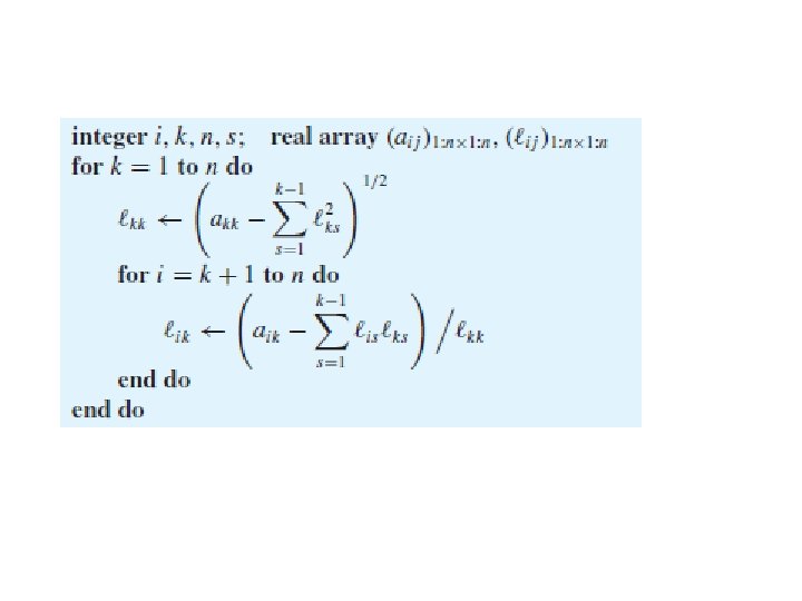
Cholesky Factorization • Any symmetric matrix that has an LU factorization in which L is unit lower triangular, has an LDLT factorization • Cholesky factorization A = LLT • case A - symmetric and positive definite.

• • A = LU matrix L lower triangular and matrix U upper triangular When L is unit lower triangular, Doolittle factorization. When U is unit upper triangular, Crout factorization A - symmetric positive definite and U = LT Cholesky factorization.

• THEOREM 2 CHOLESKY THEOREM ON LLT FACTORIZATION • If A is a real, symmetric, and positive definite matrix, then it has a unique factorization, • A = LLT , in which L is lower triangular with a positive diagonal.

• a matrix A is symmetric and positive definite if A = AT and x. TAx > 0 • for every nonzero vector x • A is nonsingular • A obviously cannot map any nonzero vector into 0

• Moreover, by considering special vectors of the form • x = (x 1, x 2, . . . , xk , 0, 0, . . . , 0)T , we see that the leading principal minors of A are also positive definite • Theorem 1 implies that A has an LU decomposition • By the symmetry of A, , A = LDLT. • D - positive definite, and • its elements dii positive. • D 1/2 – diagonal matrix - diagonal elements: √dii, • Cholesky factorization.

• algorithm Cholesky factorization - special case of the general LU factorization algorithm • If A is real, symmetric, and positive definite • then by Theorem 2, • it has a unique factorization of the form A = LLT, – L lower triangular and has positive diagonal • in equation A = LU, U = LT. • In the kth step of the general algorithm, the diagonal entry is computed:

• Theorem 2 guarantees that lkk > 0. • Equation (22) gives following bound: • from which we conclude that • any element of L is bounded by the square root of a corresponding diagonal element in A • implies that the elements of L do not become large relative to A even without any pivoting

Example • Determine the Cholesky factorization of the matrix in previous exaample.

Solution • Using the results from previous example

Multiple Right-Hand Sides • Many software packages for solving linear systems allow the input of multiple right-hand sides • n × m matrix B: • each column - right-hand side of the m linear systems • for 1 j m:

• procedure Gauss used once to produce a factorization of A • procedure Solve can be used m times with righthand side vectors b( j ) to find the m solution vectors x ( j ) for 1 j m • factorization phase done in (1/3)n 3 long operations • each back substitution phases requires n 2 long operations, • this entire process done in (1/3)n 3 + mn 2 long operations. • much less than m ((1/3)n 3 + n 2)

Computing A− 1 • • some applications – statistics compute inverse of a matrix A can be done - procedures Gauss and Solve If an n × n matrix A has an inverse, it is an n × n matrix X:

• x( j ) - j th column of X • I ( j ) - j th column of I, • (23): • written as n linear systems of equations • use procedure Gauss once to produce a factorization of A, Solve n times with the right-hand side vectors I ( j ) 1 j n. • equivalent to solving, one at a time, for the columns of A− 1 x( j )

• on computing the inverse of a matrix • In solving a linear system Ax = b, • not advisable to determine A− 1 and then compute the matrix-vector product • x = A− 1 b • requires many unnecessary calculations, compared to directly solving Ax = b for x

Example Using Software Packages • • A permutation matrix: n×n matrix P arises from the identity matrix by permuting its rows permuting the rows of any n×n matrix A can be accomplished by multiplying A on the left by P. Every permutation matrix is nonsingular the rows still form a basis for Rn When Gaussian elimination with row pivoting is performed on a matrix A, PA = LU where L: lower triangular and U: upper triangular

• The matrix PA is A with its rows rearranged • LU factorization of PA, how to solve the system Ax = b? • First, write: PAx = Pb • then LUx = Pb • Let y = Ux, so that L y = Pb Ux = y

• The first equati is easily solved for y, • and then the second equation is easily solved for x • Mathematical software systems such as Matlab, Maple, and Mathematica produce • factorizations of the form PA = LU upon command.

Example • Use mathematical software systems such as Matlab, Maple, and Mathematica to find the • LU factorization of this matrix:

Solution • Maple and find this factorization:

• Next, use Matlab and find a different factorization: • P permutation matrix corresponding to the pivoting strategy used

• Finally, use Mathematica to create this LU decomposition: • output is in a compact store scheme that contains both the lower triangular matrix • and the upper triangular matrix in a single matrix