CSE 480 Database Systems Lecture 22 Query Optimization

CSE 480: Database Systems Lecture 22: Query Optimization Reference: Read Chapter 15. 6 – 15. 8 of the textbook 1

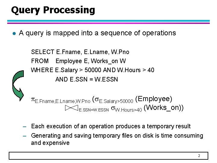
Query Processing l A query is mapped into a sequence of operations SELECT E. Fname, E. Lname, W. Pno FROM Employee E, Works_on W WHERE E. Salary > 50000 AND W. Hours > 40 AND E. SSN = W. ESSN E. Fname, E. Lname, W. Pno ( E. Salary>50000 (Employee) E. SSN=W. ESSN W. Hours>40 (Works_on)) – Each execution of an operation produces a temporary result – Generating and saving temporary files on disk is time consuming and expensive 2

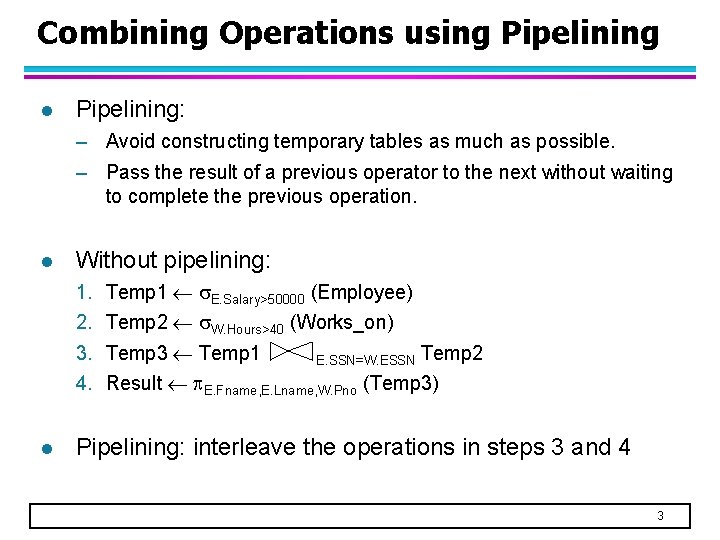
Combining Operations using Pipelining l Pipelining: – Avoid constructing temporary tables as much as possible. – Pass the result of a previous operator to the next without waiting to complete the previous operation. l Without pipelining: 1. 2. 3. 4. l Temp 1 E. Salary>50000 (Employee) Temp 2 W. Hours>40 (Works_on) Temp 3 Temp 1 E. SSN=W. ESSN Temp 2 Result E. Fname, E. Lname, W. Pno (Temp 3) Pipelining: interleave the operations in steps 3 and 4 3

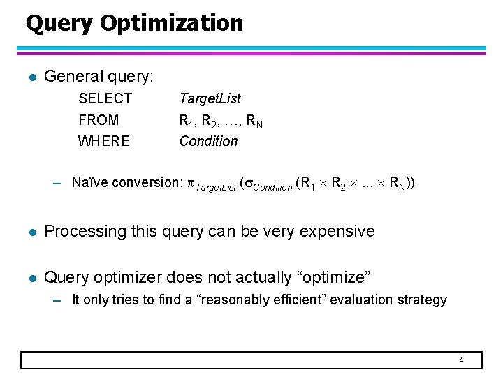
Query Optimization l General query: SELECT Target. List FROM R 1, R 2, …, RN WHERE Condition – Naïve conversion: Target. List ( Condition (R 1 R 2 . . . RN)) l Processing this query can be very expensive l Query optimizer does not actually “optimize” – It only tries to find a “reasonably efficient” evaluation strategy 4

How Does Query Optimization Work? l Uses a combination of two approaches: – Heuristic rules (on query trees) – Cost-based estimation 5

Query Tree l A relational algebra expression can be represented by a query tree – Leaf nodes are input relations of the query – Internal nodes represent relational algebra operations l A query tree can be “executed” – Execute an internal node operation whenever its operands are available and then replace the internal node by the relation that results from executing the operation 6

Example For every project located in ‘Stafford’, retrieve the project number, the controlling department number, and the department manager’s last name, address, and birth date l SQL: SELECT P. Pnumber, P. Dnum, E. Lname, E. Address, E. Bdate FROM PROJECT P, DEPARTMENT D, EMPLOYEE E WHERE P. Dnum = D. Dnumber AND D. Mgr_ssn = E. SSN AND P. Plocation = ‘Stafford’; l Relational algebra (naïve conversion): PNUMBER, DNUM, LNAME, ADDRESS, BDATE ( PLOCATION=‘STAFFORD’ AND DNUM=DNUMBER AND MGRSSN=SSN ( PROJECT DEPARTMENT EMPLOYEE)) 7

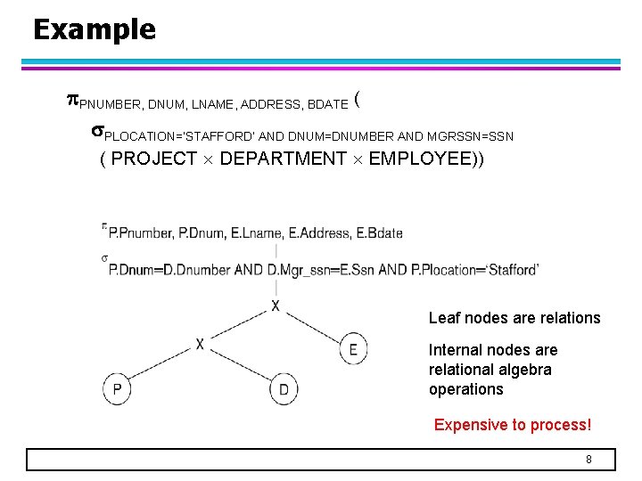
Example PNUMBER, DNUM, LNAME, ADDRESS, BDATE ( PLOCATION=‘STAFFORD’ AND DNUM=DNUMBER AND MGRSSN=SSN ( PROJECT DEPARTMENT EMPLOYEE)) Leaf nodes are relations Internal nodes are relational algebra operations Expensive to process! 8

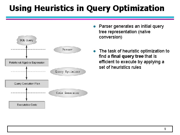
Using Heuristics in Query Optimization l Parser generates an initial query tree representation (naïve conversion) l The task of heuristic optimization to find a final query tree that is efficient to execute by applying a set of heuristics rules 9

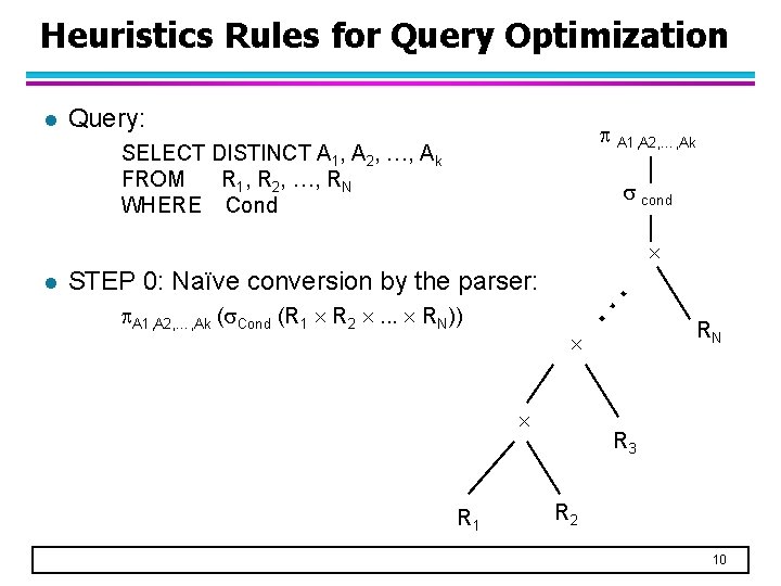
Heuristics Rules for Query Optimization l Query: A 1, A 2, …, Ak SELECT DISTINCT A 1, A 2, …, Ak FROM R 1, R 2, …, RN WHERE Cond cond l STEP 0: Naïve conversion by the parser: A 1, A 2, …, Ak ( Cond (R 1 R 2 . . . RN)) … R 1 RN R 3 R 2 10

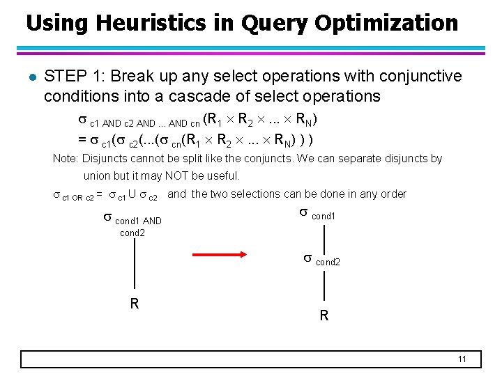
Using Heuristics in Query Optimization l STEP 1: Break up any select operations with conjunctive conditions into a cascade of select operations c 1 AND c 2 AND. . . AND cn (R 1 R 2 . . . RN) = c 1( c 2(. . . ( cn(R 1 R 2 . . . RN) ) ) Note: Disjuncts cannot be split like the conjuncts. We can separate disjuncts by union but it may NOT be useful. c 1 OR c 2 = c 1 U c 2 and the two selections can be done in any order cond 1 AND cond 1 cond 2 R R 11

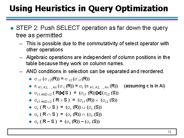
Using Heuristics in Query Optimization l STEP 2: Push SELECT operation as far down the query tree as permitted – This is possible due to the commutativity of select operator with other operations – Algebraic operations are independent of column positions in the table because they work on column names. – AND conditions in selection can be separated and reordered. u c 1 ( c 2(R)) = c 2 ( c 1(R)) u A 1, A 2, . . . , An ( c (R)) = c ( A 1, A 2, . . . , An (R)) u c 1 AND c 2 ( R S ) = ( c 1 (R)) ( c 2 (S)) u c ( R S ) = ( c (R)) ( c (S)) u c ( R – S ) = ( c (R)) – ( c (S)) S ) = ( c 1 (R)) (assuming c is in Ai) ( c 2 (S)) 12

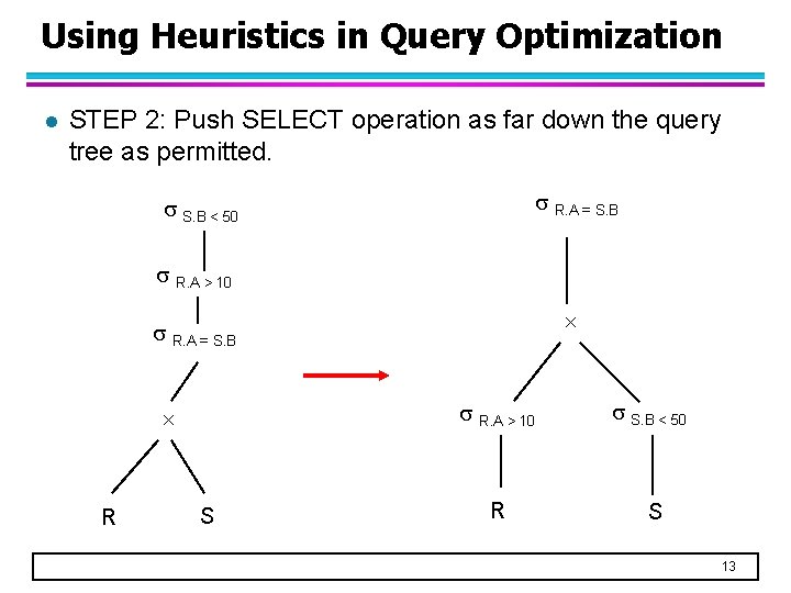
Using Heuristics in Query Optimization l STEP 2: Push SELECT operation as far down the query tree as permitted. R. A = S. B < 50 R. A > 10 R. A = S. B R S R. A > 10 S. B < 50 R S 13

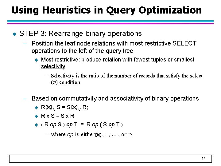
Using Heuristics in Query Optimization l STEP 3: Rearrange binary operations – Position the leaf node relations with most restrictive SELECT operations to the left of the query tree u Most restrictive: produce relation with fewest tuples or smallest selectivity – Selectivity is the ratio of the number of records that satisfy the select ( ) condition – Based on commutativity and associativity of binary operations u Rx. S=Sx. R u ( R op S ) op T = R op ( S op T ) C S=S C R; – where op is either , , , or 14

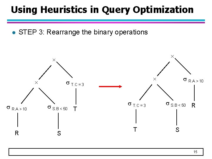
Using Heuristics in Query Optimization l STEP 3: Rearrange the binary operations R. A > 10 R T. C = 3 S. B < 50 T S T. C = 3 T R. A > 10 S. B < 50 R S 15

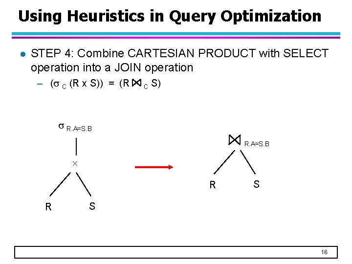
Using Heuristics in Query Optimization l STEP 4: Combine CARTESIAN PRODUCT with SELECT operation into a JOIN operation – ( C (R x S)) = (R C S) R. A=S. B R R S S 16

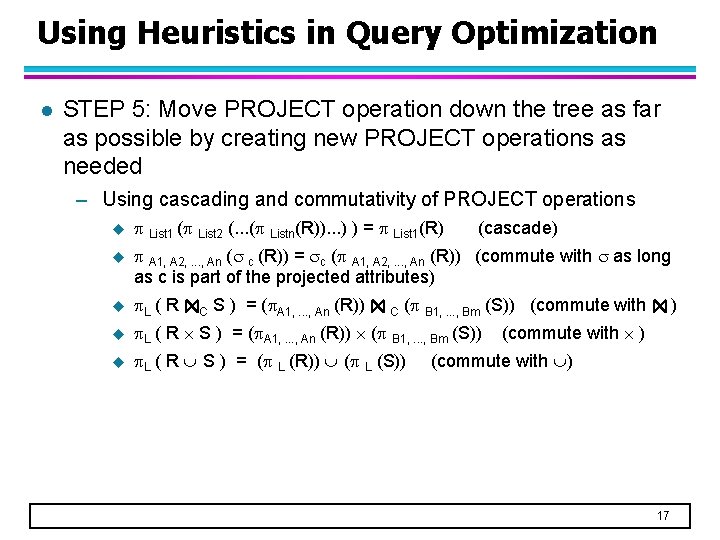
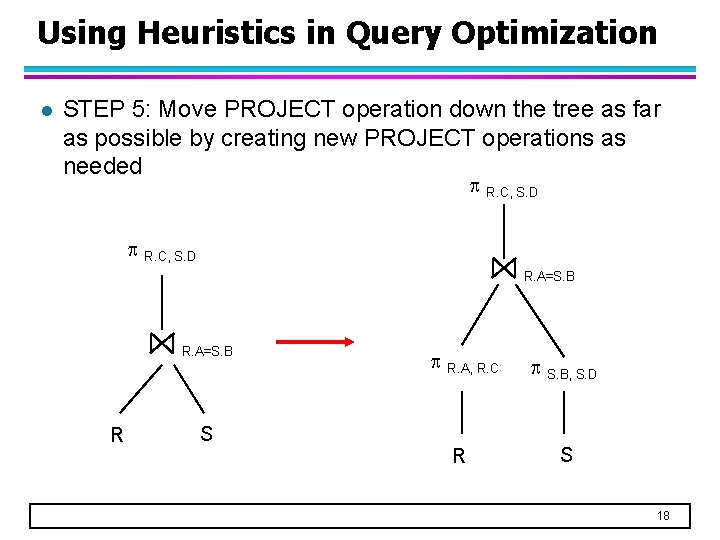
Using Heuristics in Query Optimization l STEP 5: Move PROJECT operation down the tree as far as possible by creating new PROJECT operations as needed – Using cascading and commutativity of PROJECT operations u List 1 ( List 2 (. . . ( Listn(R)). . . ) ) = List 1(R) u A 1, A 2, . . . , An ( c (R)) = c ( A 1, A 2, . . . , An (R)) (commute with as long as c is part of the projected attributes) u L ( R S ) = ( A 1, . . . , An (R)) ( B 1, . . . , Bm (S)) u L ( R S ) = ( L (R)) ( L (S)) C S ) = ( A 1, . . . , An (R)) C (cascade) ( B 1, . . . , Bm (S)) (commute with ) 17

Using Heuristics in Query Optimization l STEP 5: Move PROJECT operation down the tree as far as possible by creating new PROJECT operations as needed R. C, S. D R. A=S. B R S R. A, R. C R S. B, S. D S 18

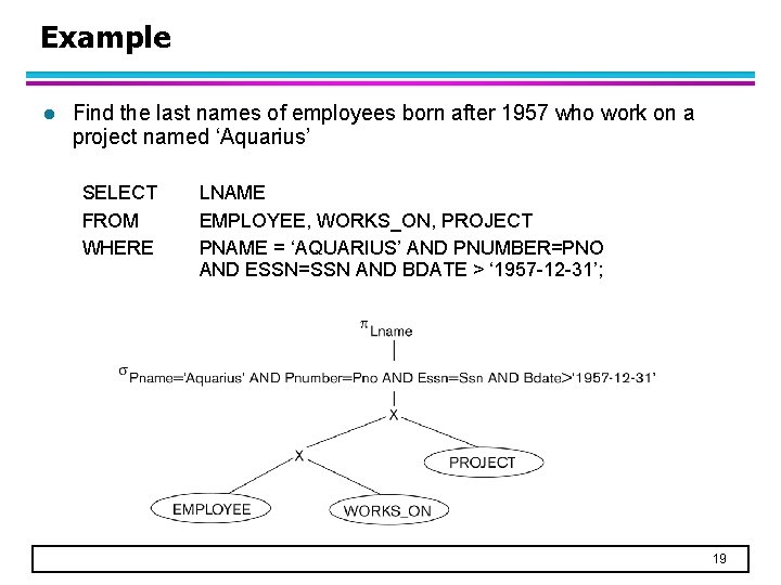
Example l Find the last names of employees born after 1957 who work on a project named ‘Aquarius’ SELECT FROM WHERE LNAME EMPLOYEE, WORKS_ON, PROJECT PNAME = ‘AQUARIUS’ AND PNUMBER=PNO AND ESSN=SSN AND BDATE > ‘ 1957 -12 -31’; 19

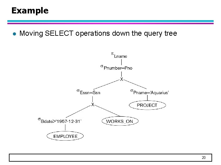
Example l Moving SELECT operations down the query tree 20

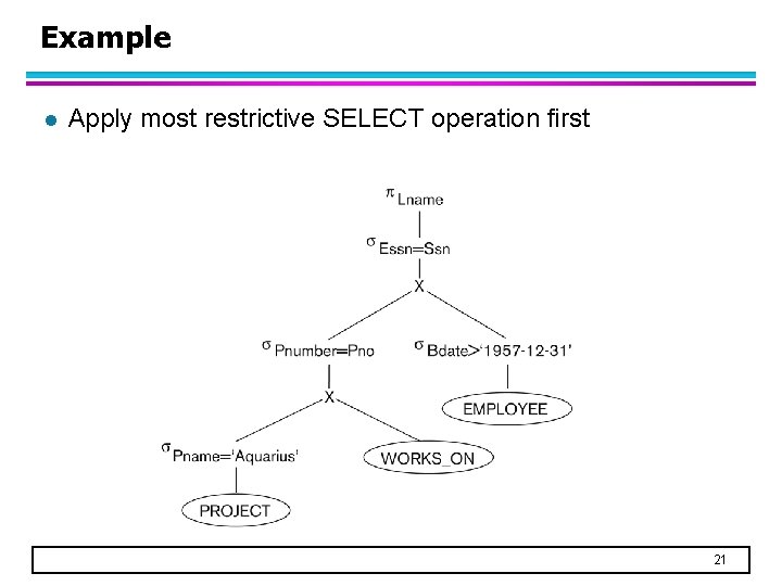
Example l Apply most restrictive SELECT operation first 21

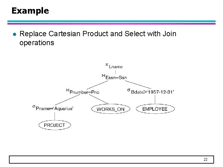
Example l Replace Cartesian Product and Select with Join operations 22

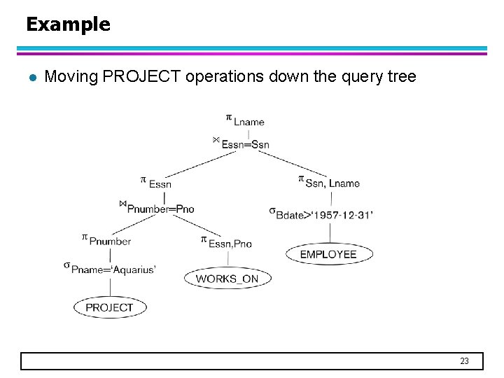
Example l Moving PROJECT operations down the query tree 23

Cost-based Query Optimization l Estimate and compare the costs of executing a query using different execution strategies and choose the strategy with the lowest cost estimate. l Example query: SELECT Pnumber, Dnum, Lname, Address, Bdate FROM PROJECT, DEPARTMENT, EMPLOYEE WHERE Dnum = Dnumber AND Mgr_ssn = Ssn AND Plocation = ‘Stafford’ 24

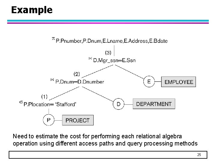
Example Need to estimate the cost for performing each relational algebra operation using different access paths and query processing methods 25

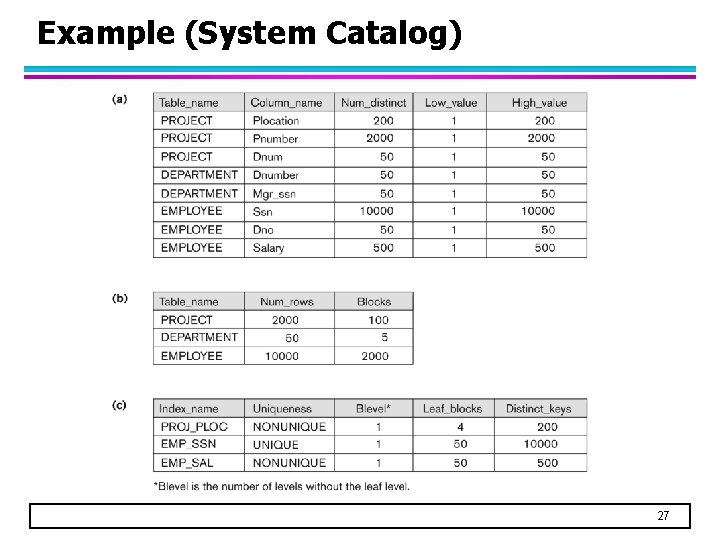
Cost-based Query Optimization l System Catalog Information – Information about the size of a file u number of records (tuples) (r), u record size (R), u number of blocks (b) u blocking factor (bfr) number of records per block – Information about indexes and indexing attributes of a file u Number of levels (x) of each multilevel index u Number of first-level index blocks (b. I 1) u Number of distinct values (d) of an attribute u Selectivity (sl) of an attribute 26

Example (System Catalog) 27

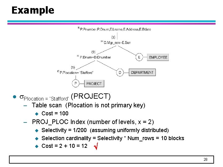
Example l Plocation = ‘Stafford’ (PROJECT) – Table scan (Plocation is not primary key) u Cost = 100 – PROJ_PLOC Index (number of levels, x = 2) u u u Selectivity = 1/200 (assuming uniformly distributed) Selection cardinality = Selectivity * Num_rows = 10 blocks Cost = 2 + 10 = 12 28

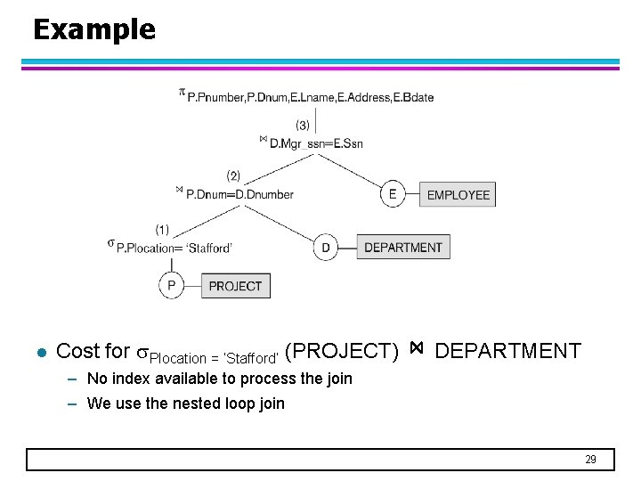
Example l Cost for Plocation = ‘Stafford’ (PROJECT) DEPARTMENT – No index available to process the join – We use the nested loop join 29

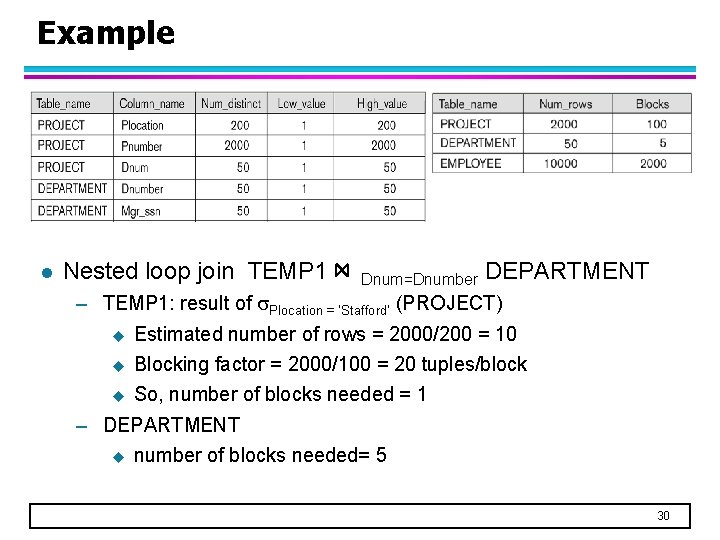
Example l Nested loop join TEMP 1 Dnum=Dnumber DEPARTMENT – TEMP 1: result of Plocation = ‘Stafford’ (PROJECT) u Estimated number of rows = 2000/200 = 10 u Blocking factor = 2000/100 = 20 tuples/block u So, number of blocks needed = 1 – DEPARTMENT u number of blocks needed= 5 30

Example l Nested loop join TEMP 1 Dnum=Dnumber DEPARTMENT – Use TEMP 1 in outer loop for nested-loop join u Cost = 1 + 5 + cost to write join output into TEMP 2 = 6 + cost to write join output into TEMP 2 – What is the cost for writing join output? u Each row in TEMP 1 joins exactly 1 row in DEPARTMENT u Estimated number of rows in TEMP 2 = 10 (join attribute dno is the key of department. So we assume there are 10 joined records) u Estimated blocking factor = 5 (from estimated record size) u Number of blocks needed = 2 31

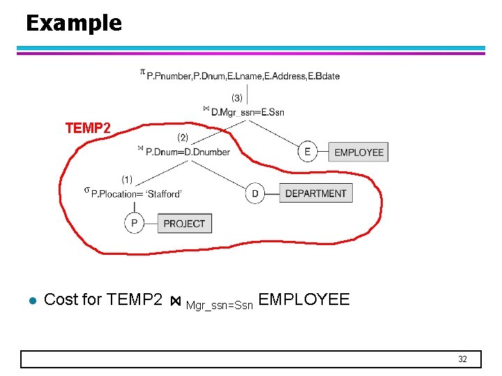
Example TEMP 2 l Cost for TEMP 2 Mgr_ssn=Ssn EMPLOYEE 32

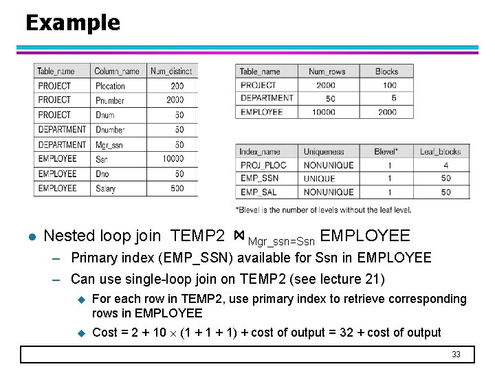
Example l Nested loop join TEMP 2 Mgr_ssn=Ssn EMPLOYEE – Primary index (EMP_SSN) available for Ssn in EMPLOYEE – Can use single-loop join on TEMP 2 (see lecture 21) u For each row in TEMP 2, use primary index to retrieve corresponding rows in EMPLOYEE u Cost = 2 + 10 (1 + 1) + cost of output = 32 + cost of output 33

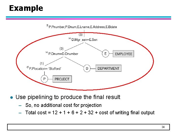
Example l Use pipelining to produce the final result – So, no additional cost for projection – Total cost = 12 + 1 + 6 + 2 + 32 + cost of writing final output 34

Query Execution Plan l An execution plan consists of a combination of – The relational algebra query tree and – Information about how to compute the relational operators in the tree u Based on the access paths and algorithms available l Generated by the query optimizer module in DBMS – A code generator then generates the code to execute the plan – Finally, the runtime database processor will execute the code (either in compiled or interpreted mode) to produce the query result 35