CSE 473 Artificial Intelligence Spring 2012 Bayesian Networks
CSE 473: Artificial Intelligence Spring 2012 Bayesian Networks - Learning Dan Weld Slides adapted from Jack Breese, Dan Klein, Daphne Koller, Stuart Russell, Andrew Moore & Luke Zettlemoyer 1
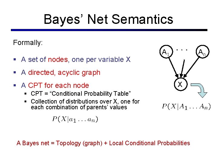
Bayes’ Net Semantics Formally: § A set of nodes, one per variable X A 1 An § A directed, acyclic graph § A CPT for each node X § CPT = “Conditional Probability Table” § Collection of distributions over X, one for each combination of parents’ values A Bayes net = Topology (graph) + Local Conditional Probabilities
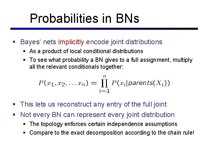
Probabilities in BNs § Bayes’ nets implicitly encode joint distributions § As a product of local conditional distributions § To see what probability a BN gives to a full assignment, multiply all the relevant conditionals together: § This lets us reconstruct any entry of the full joint § Not every BN can represent every joint distribution § The topology enforces certain independence assumptions § Compare to the exact decomposition according to the chain rule!
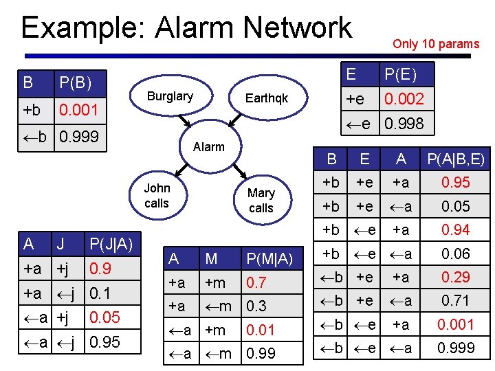
Example: Alarm Network B P(B) +b 0. 001 Burglary Earthqk Alarm John calls J +a +j P(J|A) 0. 9 +a ¬j 0. 1 ¬a +j 0. 05 ¬a ¬j 0. 95 E P(E) +e 0. 002 ¬e 0. 998 ¬b 0. 999 A Only 10 params Mary calls A M P(M|A) +a +m 0. 7 +a ¬m 0. 3 ¬a +m 0. 01 ¬a ¬m 0. 99 B E A P(A|B, E) +b +e +a 0. 95 +b +e ¬a 0. 05 +b ¬e +a 0. 94 +b ¬e ¬a 0. 06 ¬b +e +a 0. 29 ¬b +e ¬a 0. 71 ¬b ¬e +a 0. 001 ¬b ¬e ¬a 0. 999
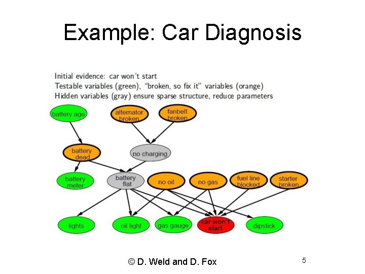
Example: Car Diagnosis © D. Weld and D. Fox 5
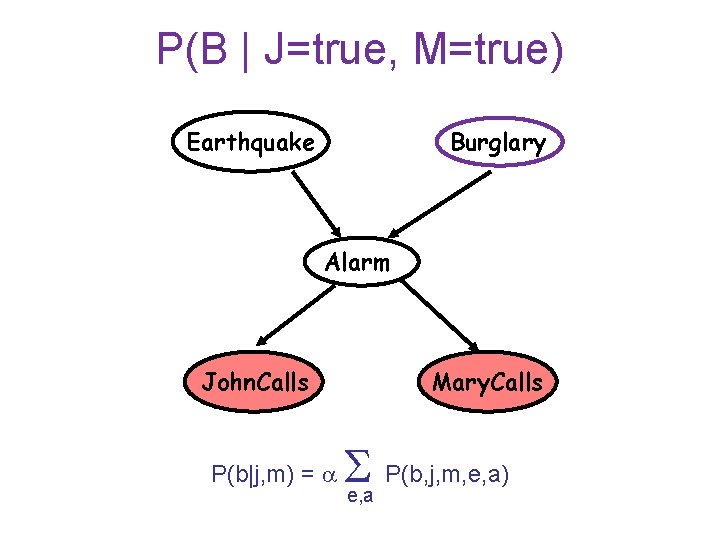
P(B | J=true, M=true) Earthquake Burglary Alarm John. Calls P(b|j, m) = Mary. Calls P(b, j, m, e, a) e, a
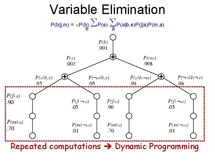
Variable Elimination P(b|j, m) = P(b) e P(e) a P(a|b, e)P(j|a)P(m, a) Repeated computations Dynamic Programming
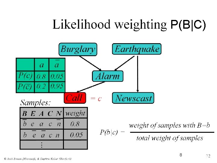
P(B|C) 8

MCMC with Gibbs Sampling § § § Fix the values of observed variables Set the values of all non-observed variables randomly Perform a random walk through the space of complete variable assignments. On each move: 1. Pick a variable X 2. Calculate Pr(X=true | Markov blanket) 3. Set X to true with that probability Repeat many times. Frequency with which any variable X is true is it’s posterior probability. Converges to true posterior when frequencies stop changing significantly § stable distribution, mixing 9

The Origin of Bayes Nets Earthquake Radio Nbr 1 Calls © Daniel S. Weld Burglary Alarm e, b Pr(B=t) Pr(B=f) 0. 05 0. 95 Pr(A|E, B) 0. 9 (0. 1) 0. 2 (0. 8) 0. 85 (0. 15) 0. 01 (0. 99) Nbr 2 Calls 10
Learning Topics § Learning Parameters for a Bayesian Network § Fully observable § Maximum Likelihood (ML) § Maximum A Posteriori (MAP) § Bayesian § Hidden variables (EM algorithm) § Learning Structure of Bayesian Networks © Daniel S. Weld

Parameter Estimation and Bayesian Networks E B R A J M T F T F F F T F T T T F F F F We have: . . . - Bayes Net structure and observations - We need: Bayes Net parameters
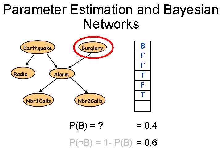
Parameter Estimation and Bayesian Networks E T F F B F F T R T F F . . . P(B) = ? = 0. 4 P(¬B) = 1 - P(B) = 0. 6 A T F T T F J F F T T F M T T F

Parameter Estimation and Bayesian Networks E T F F. . . P(A|E, B) = ? P(A|E, ¬B) = ? P(A|¬E, ¬B) = ? B F F T R T F F A T F T T F J F F T T F M T T F
Parameter Estimation and Bayesian Networks Coin
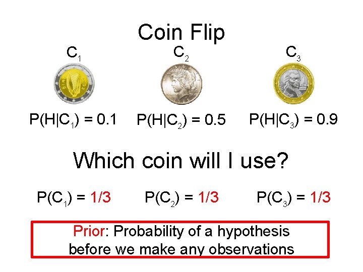
C 1 P(H|C 1) = 0. 1 Coin Flip C 2 C 3 P(H|C 2) = 0. 5 P(H|C 3) = 0. 9 Which coin will I use? P(C 1) = 1/3 P(C 2) = 1/3 P(C 3) = 1/3 Prior: Probability of a hypothesis before we make any observations
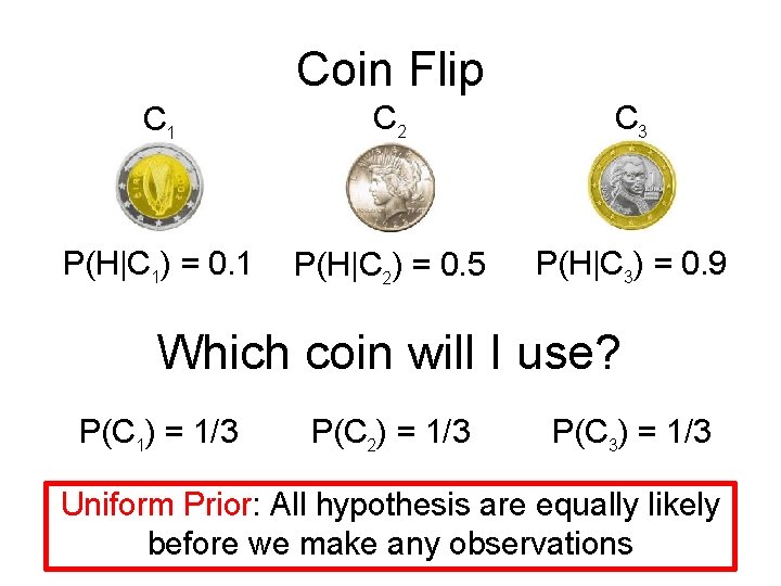
Coin Flip C 1 C 2 C 3 P(H|C 1) = 0. 1 P(H|C 2) = 0. 5 P(H|C 3) = 0. 9 Which coin will I use? P(C 1) = 1/3 P(C 2) = 1/3 P(C 3) = 1/3 Uniform Prior: All hypothesis are equally likely before we make any observations
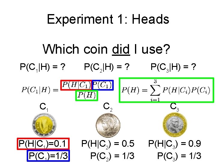
Experiment 1: Heads Which coin did I use? P(C 1|H) = ? P(C 2|H) = ? P(C 3|H) = ? C 1 C 2 C 3 P(H|C 1)=0. 1 P(C 1)=1/3 P(H|C 2) = 0. 5 P(C 2) = 1/3 P(H|C 3) = 0. 9 P(C 3) = 1/3
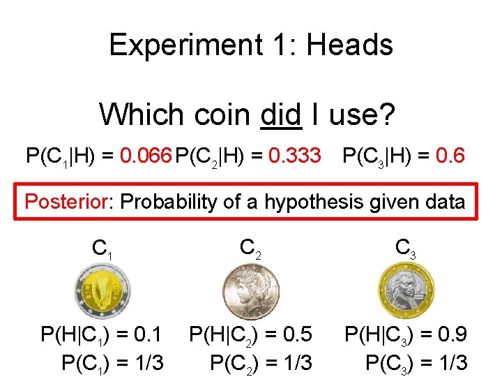
Experiment 1: Heads Which coin did I use? P(C 1|H) = 0. 066 P(C 2|H) = 0. 333 P(C 3|H) = 0. 6 Posterior: Probability of a hypothesis given data C 1 C 2 C 3 P(H|C 1) = 0. 1 P(C 1) = 1/3 P(H|C 2) = 0. 5 P(C 2) = 1/3 P(H|C 3) = 0. 9 P(C 3) = 1/3
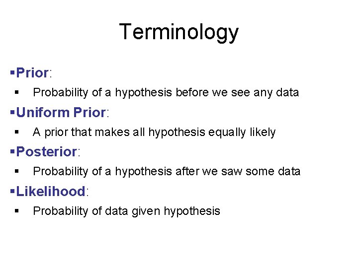
Terminology §Prior: § Probability of a hypothesis before we see any data §Uniform Prior: § A prior that makes all hypothesis equally likely §Posterior: § Probability of a hypothesis after we saw some data §Likelihood: § Probability of data given hypothesis
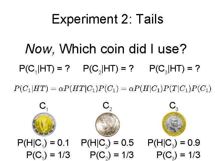
Experiment 2: Tails Now, Which coin did I use? P(C 1|HT) = ? P(C 2|HT) = ? P(C 3|HT) = ? C 1 C 2 C 3 P(H|C 1) = 0. 1 P(C 1) = 1/3 P(H|C 2) = 0. 5 P(C 2) = 1/3 P(H|C 3) = 0. 9 P(C 3) = 1/3
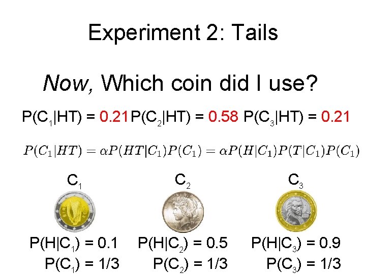
Experiment 2: Tails Now, Which coin did I use? P(C 1|HT) = 0. 21 P(C 2|HT) = 0. 58 P(C 3|HT) = 0. 21 C 2 C 3 P(H|C 1) = 0. 1 P(C 1) = 1/3 P(H|C 2) = 0. 5 P(C 2) = 1/3 P(H|C 3) = 0. 9 P(C 3) = 1/3
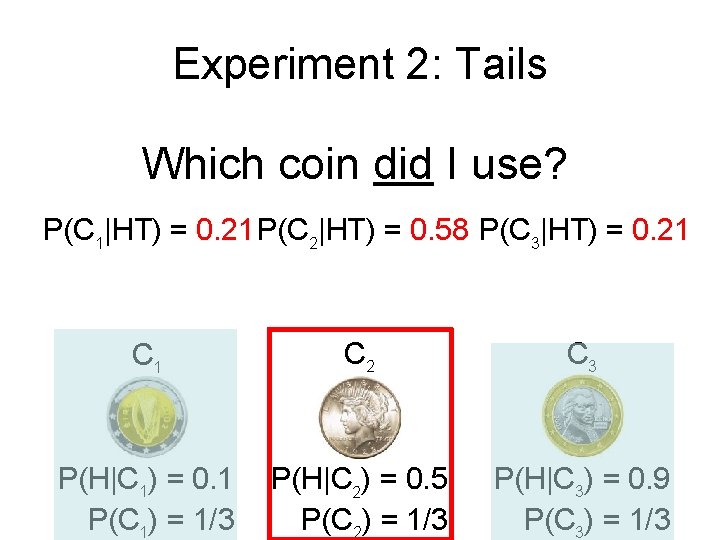
Experiment 2: Tails Which coin did I use? P(C 1|HT) = 0. 21 P(C 2|HT) = 0. 58 P(C 3|HT) = 0. 21 C 2 C 3 P(H|C 1) = 0. 1 P(C 1) = 1/3 P(H|C 2) = 0. 5 P(C 2) = 1/3 P(H|C 3) = 0. 9 P(C 3) = 1/3
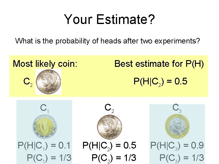
Your Estimate? What is the probability of heads after two experiments? Most likely coin: Best estimate for P(H) C 2 P(H|C 2) = 0. 5 C 1 C 2 C 3 P(H|C 1) = 0. 1 P(C 1) = 1/3 P(H|C 2) = 0. 5 P(C 2) = 1/3 P(H|C 3) = 0. 9 P(C 3) = 1/3
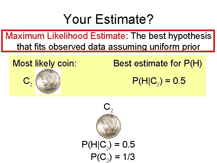
Your Estimate? Maximum Likelihood Estimate: The best hypothesis that fits observed data assuming uniform prior Most likely coin: Best estimate for P(H) C 2 P(H|C 2) = 0. 5 P(C 2) = 1/3
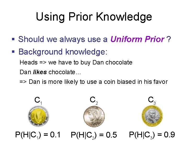
Using Prior Knowledge § Should we always use a Uniform Prior ? § Background knowledge: Heads => we have to buy Dan chocolate Dan likes chocolate… => Dan is more likely to use a coin biased in his favor C 1 C 2 C 3 P(H|C 1) = 0. 1 P(H|C 2) = 0. 5 P(H|C 3) = 0. 9
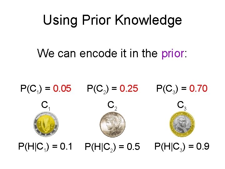
Using Prior Knowledge We can encode it in the prior: P(C 1) = 0. 05 P(C 2) = 0. 25 P(C 3) = 0. 70 C 1 C 2 C 3 P(H|C 1) = 0. 1 P(H|C 2) = 0. 5 P(H|C 3) = 0. 9
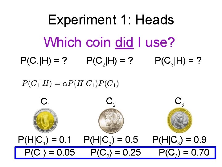
Experiment 1: Heads Which coin did I use? P(C 1|H) = ? P(C 2|H) = ? P(C 3|H) = ? C 1 C 2 C 3 P(H|C 1) = 0. 1 P(H|C 2) = 0. 5 P(C 1) = 0. 05 P(C 2) = 0. 25 P(H|C 3) = 0. 9 P(C 3) = 0. 70
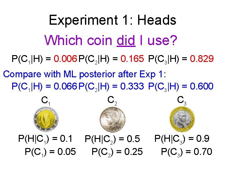
Experiment 1: Heads Which coin did I use? P(C 1|H) = 0. 006 P(C 2|H) = 0. 165 P(C 3|H) = 0. 829 Compare with ML posterior after Exp 1: P(C 1|H) = 0. 066 P(C 2|H) = 0. 333 P(C 3|H) = 0. 600 C 2 C 3 C 1 P(H|C 1) = 0. 1 P(H|C 2) = 0. 5 P(C 1) = 0. 05 P(C 2) = 0. 25 P(H|C 3) = 0. 9 P(C 3) = 0. 70
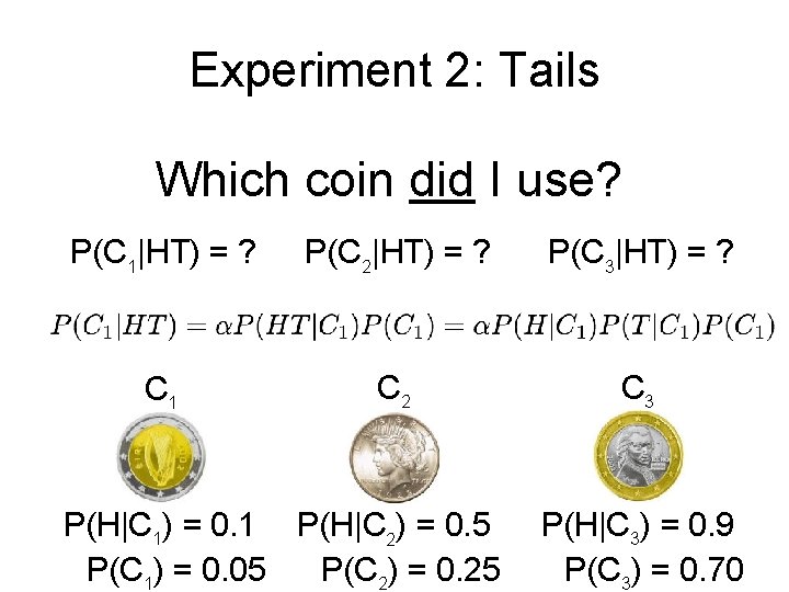
Experiment 2: Tails Which coin did I use? P(C 1|HT) = ? P(C 2|HT) = ? P(C 3|HT) = ? C 1 C 2 C 3 P(H|C 1) = 0. 1 P(H|C 2) = 0. 5 P(C 1) = 0. 05 P(C 2) = 0. 25 P(H|C 3) = 0. 9 P(C 3) = 0. 70
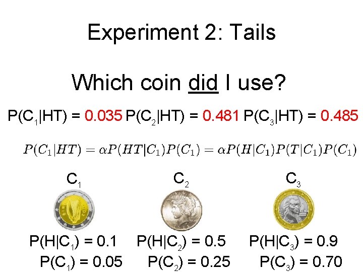
Experiment 2: Tails Which coin did I use? P(C 1|HT) = 0. 035 P(C 2|HT) = 0. 481 P(C 3|HT) = 0. 485 C 1 C 2 P(H|C 1) = 0. 1 P(H|C 2) = 0. 5 P(C 1) = 0. 05 P(C 2) = 0. 25 C 3 P(H|C 3) = 0. 9 P(C 3) = 0. 70
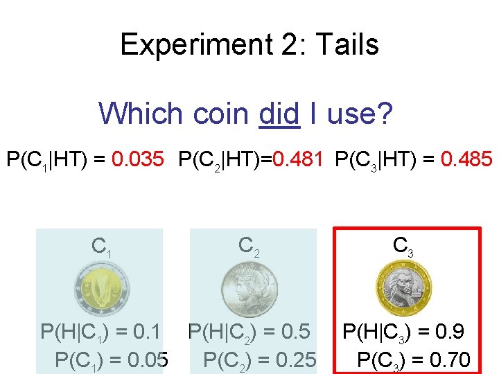
Experiment 2: Tails Which coin did I use? P(C 1|HT) = 0. 035 P(C 2|HT)=0. 481 P(C 3|HT) = 0. 485 C 1 C 2 P(H|C 1) = 0. 1 P(H|C 2) = 0. 5 P(C 1) = 0. 05 P(C 2) = 0. 25 C 3 P(H|C 3) = 0. 9 P(C 3) = 0. 70
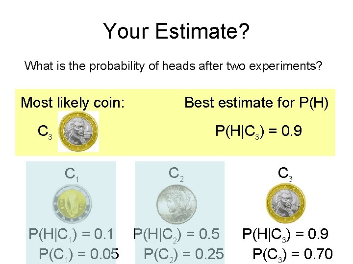
Your Estimate? What is the probability of heads after two experiments? Most likely coin: Best estimate for P(H) C 3 P(H|C 3) = 0. 9 C 1 C 2 P(H|C 1) = 0. 1 P(H|C 2) = 0. 5 P(C 1) = 0. 05 P(C 2) = 0. 25 C 3 P(H|C 3) = 0. 9 P(C 3) = 0. 70
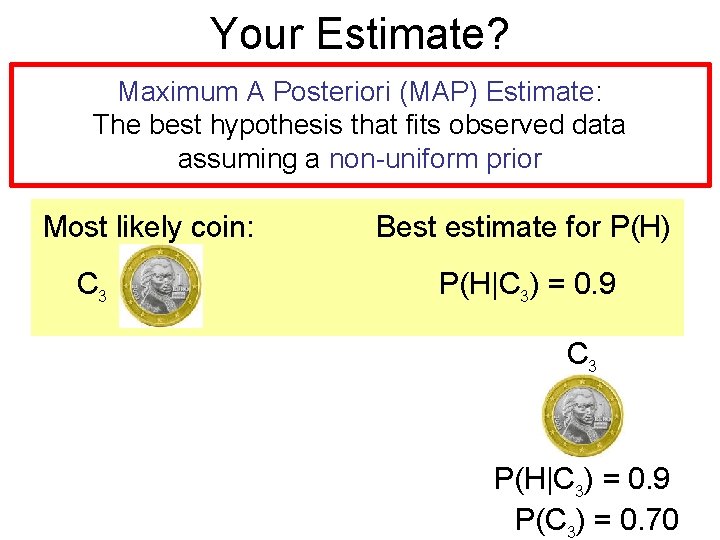
Your Estimate? Maximum A Posteriori (MAP) Estimate: The best hypothesis that fits observed data assuming a non-uniform prior Most likely coin: C 3 Best estimate for P(H) P(H|C 3) = 0. 9 C 3 P(H|C 3) = 0. 9 P(C 3) = 0. 70
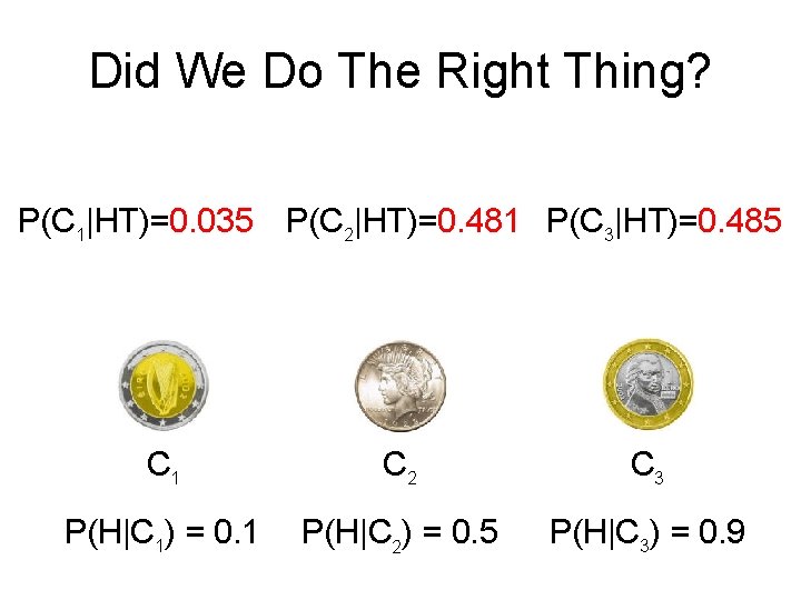
Did We Do The Right Thing? P(C 1|HT)=0. 035 P(C 2|HT)=0. 481 P(C 3|HT)=0. 485 C 1 C 2 C 3 P(H|C 1) = 0. 1 P(H|C 2) = 0. 5 P(H|C 3) = 0. 9
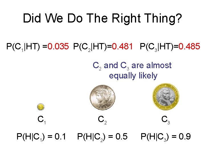
Did We Do The Right Thing? P(C 1|HT) =0. 035 P(C 2|HT)=0. 481 P(C 3|HT)=0. 485 C 2 and C 3 are almost equally likely C 1 C 2 C 3 P(H|C 1) = 0. 1 P(H|C 2) = 0. 5 P(H|C 3) = 0. 9
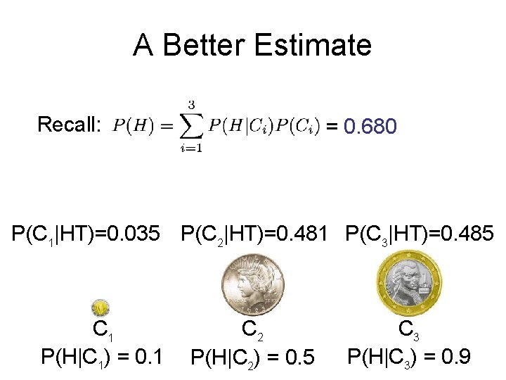
A Better Estimate Recall: = 0. 680 P(C 1|HT)=0. 035 P(C 2|HT)=0. 481 P(C 3|HT)=0. 485 C 1 P(H|C 1) = 0. 1 C 2 P(H|C 2) = 0. 5 C 3 P(H|C 3) = 0. 9
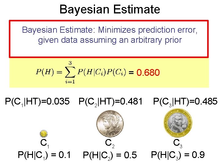
Bayesian Estimate: Minimizes prediction error, given data assuming an arbitrary prior = 0. 680 P(C 1|HT)=0. 035 P(C 2|HT)=0. 481 C 1 P(H|C 1) = 0. 1 C 2 P(H|C 2) = 0. 5 P(C 3|HT)=0. 485 C 3 P(H|C 3) = 0. 9
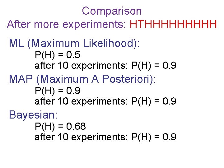
Comparison After more experiments: HTHHHHH ML (Maximum Likelihood): P(H) = 0. 5 after 10 experiments: P(H) = 0. 9 MAP (Maximum A Posteriori): P(H) = 0. 9 after 10 experiments: P(H) = 0. 9 Bayesian: P(H) = 0. 68 after 10 experiments: P(H) = 0. 9
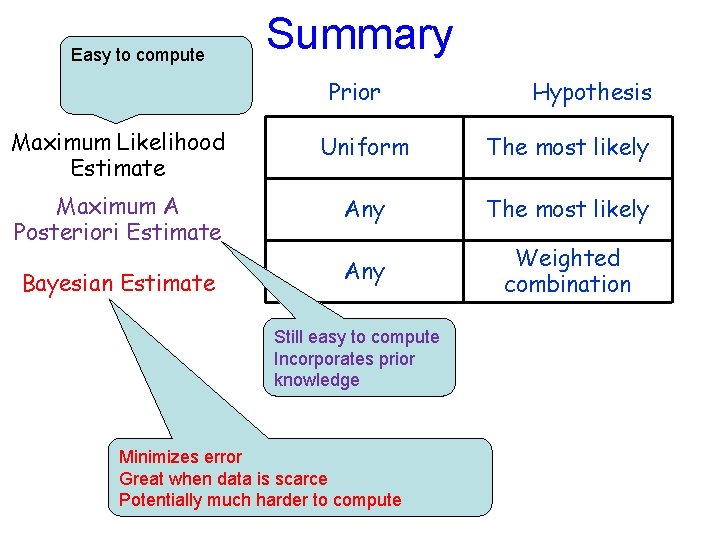
Easy to compute Summary Prior Hypothesis Maximum Likelihood Estimate Uniform The most likely Maximum A Posteriori Estimate Any The most likely Bayesian Estimate Any Weighted combination Still easy to compute Incorporates prior knowledge Minimizes error Great when data is scarce Potentially much harder to compute

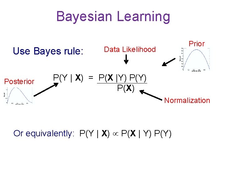
Bayesian Learning Use Bayes rule: Posterior Prior Data Likelihood P(Y | X) = P(X |Y) P(X) Normalization Or equivalently: P(Y | X) P(X | Y) P(Y)
Parameter Estimation and Bayesian Networks E T F F B F F T R T F F A T F T T F J F F T T F M T T F . . . Prior P(B) = ? + data = Now compute either MAP or Bayesian estimate
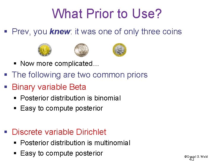
What Prior to Use? § Prev, you knew: it was one of only three coins § Now more complicated… § The following are two common priors § Binary variable Beta § Posterior distribution is binomial § Easy to compute posterior § Discrete variable Dirichlet § Posterior distribution is multinomial § Easy to compute posterior © Daniel S. Weld 43
Beta Distribution
![Beta Distribution § Example: Flip coin with Beta distribution as prior over p [prob(heads)] Beta Distribution § Example: Flip coin with Beta distribution as prior over p [prob(heads)]](http://slidetodoc.com/presentation_image_h2/73c9e3e9cfd24af9d456e4e4c45b6259/image-45.jpg)
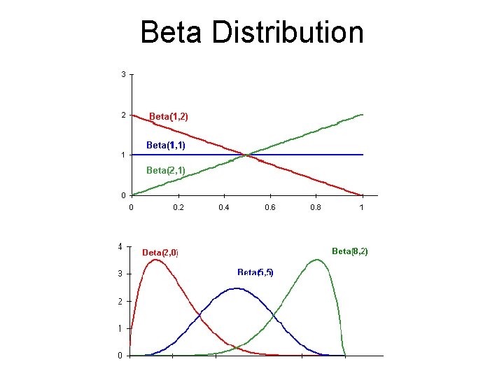
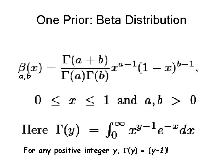
Beta Distribution § Example: Flip coin with Beta distribution as prior over p [prob(heads)] 1. 2. 3. 4. Parameterized by two positive numbers: a, b Mode of distribution (E[p]) is a/(a+b) Specify our prior belief for p = a/(a+b) Specify confidence in this belief with high initial values for a and b § Updating our prior belief based on data § incrementing a for every heads outcome § incrementing b for every tails outcome
One Prior: Beta Distribution a, b For any positive integer y, G(y) = (y-1)!
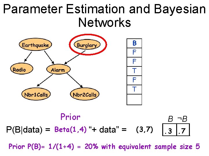
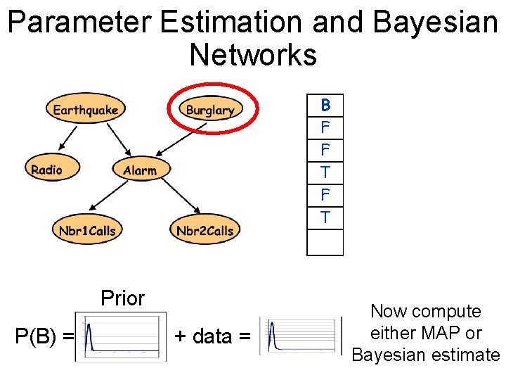
Parameter Estimation and Bayesian Networks E T F F B F F T R T F F A T F T T F J F F T T F M T T F . . . Prior P(B|data) = ? Beta(1, 4) “+ data” = B ¬B (3, 7) . 3. 7 Prior P(B)= 1/(1+4) = 20% with equivalent sample size 5
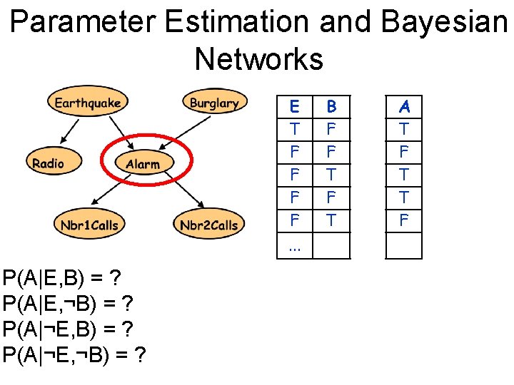
Parameter Estimation and Bayesian Networks E T F F. . . P(A|E, B) = ? P(A|E, ¬B) = ? P(A|¬E, ¬B) = ? B F F T R T F F A T F T T F J F F T T F M T T F
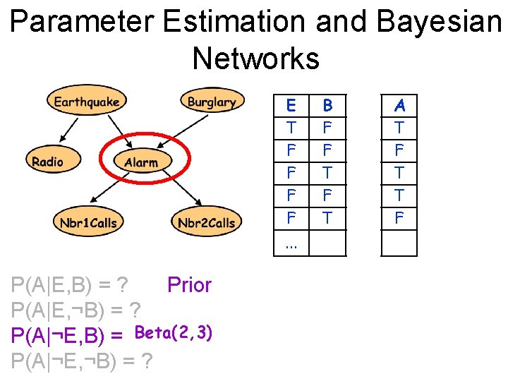
Parameter Estimation and Bayesian Networks E T F F. . . P(A|E, B) = ? Prior P(A|E, ¬B) = ? P(A|¬E, B) = ? Beta(2, 3) P(A|¬E, ¬B) = ? B F F T R T F F A T F T T F J F F T T F M T T F
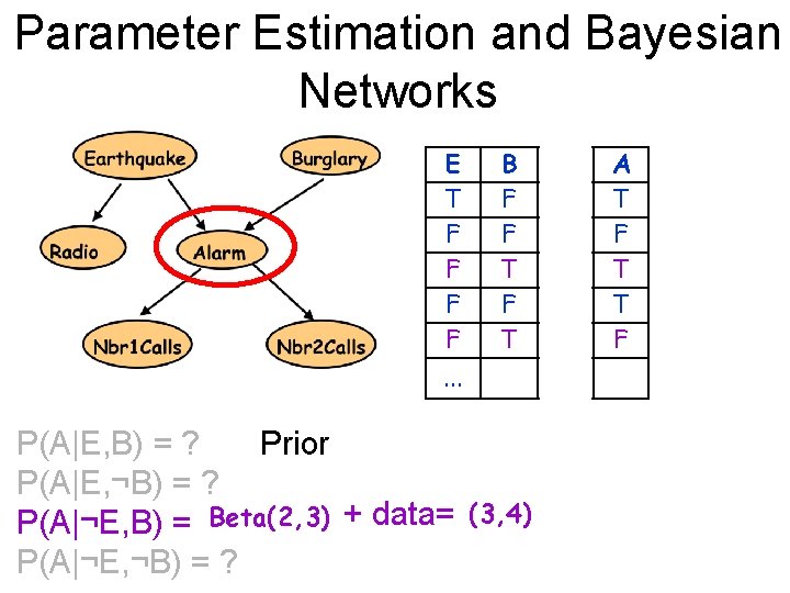
Parameter Estimation and Bayesian Networks E T F F B F F T . . . P(A|E, B) = ? Prior P(A|E, ¬B) = ? P(A|¬E, B) = ? Beta(2, 3) + data= P(A|¬E, ¬B) = ? (3, 4) R T F F A T F T T F J F F T T F M T T F
Bayesian Learning Use Bayes rule: Posterior Prior Data Likelihood P(Y | X) = P(X |Y) P(X) Normalization Or equivalently: P(Y | X) P(X | Y) P(Y)
- Slides: 51