CSE 473 Artificial Intelligence Reinforcement Learning Dan Weld

CSE 473: Artificial Intelligence Reinforcement Learning Dan Weld Many slides adapted from either Dan Klein, Stuart Russell, Luke Zettlemoyer or Andrew Moore 1

Today’s Outline § Reinforcement Learning § Q-value iteration § Q-learning § Exploration / exploitation § Linear function approximation

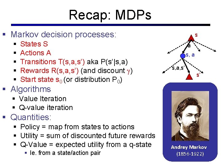
Recap: MDPs § Markov decision processes: § § § States S Actions A Transitions T(s, a, s’) aka P(s’|s, a) Rewards R(s, a, s’) (and discount ) Start state s 0 (or distribution P 0) s a s, a, s’ s’ § Algorithms § Value Iteration § Q-value iteration § Quantities: § Policy = map from states to actions § Utility = sum of discounted future rewards § Q-Value = expected utility from a q-state § Ie. from a state/action pair Andrey Markov (1856 -1922)

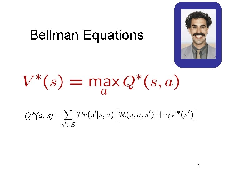
Bellman Equations Q*(a, s) = 4

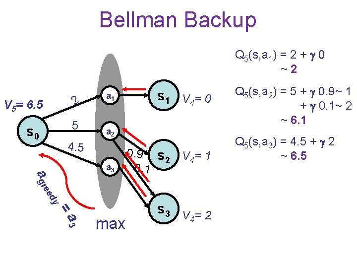
Bellman Backup Q 5(s, a 1) = 2 + 0 ~2 V 5= 6. 5 2 s 0 5 a 1 s 1 V 4= 0 a 2 4. 5 y ed a gre a 3 =a 3 max 0. 9 s 2 0. 1 V 4= 1 s 3 V = 2 4 Q 5(s, a 2) = 5 + 0. 9~ 1 + 0. 1~ 2 ~ 6. 1 Q 5(s, a 3) = 4. 5 + 2 ~ 6. 5

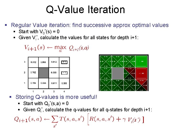
Q-Value Iteration § Regular Value iteration: find successive approx optimal values § Start with V 0*(s) = 0 § Given Vi*, calculate the values for all states for depth i+1: Qi+1(s, a) § Storing Q-values is more useful! § Start with Q 0*(s, a) = 0 § Given Qi*, calculate the q-values for all q-states for depth i+1: Vi(s’) ]

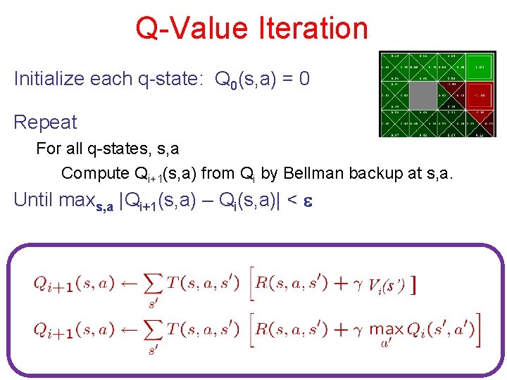
Q-Value Iteration Initialize each q-state: Q 0(s, a) = 0 Repeat For all q-states, s, a Compute Qi+1(s, a) from Qi by Bellman backup at s, a. Until maxs, a |Qi+1(s, a) – Qi(s, a)| < Vi(s’) ]

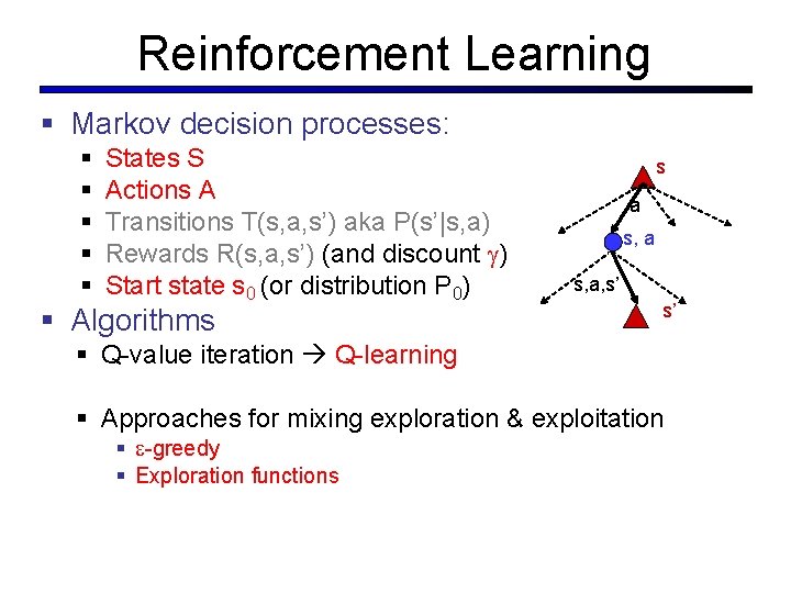
Reinforcement Learning § Markov decision processes: § § § States S Actions A Transitions T(s, a, s’) aka P(s’|s, a) Rewards R(s, a, s’) (and discount ) Start state s 0 (or distribution P 0) § Algorithms s a s, a, s’ s’ § Q-value iteration Q-learning § Approaches for mixing exploration & exploitation § -greedy § Exploration functions

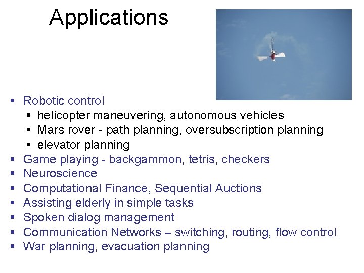
Applications § Robotic control § helicopter maneuvering, autonomous vehicles § Mars rover - path planning, oversubscription planning § elevator planning § Game playing - backgammon, tetris, checkers § Neuroscience § Computational Finance, Sequential Auctions § Assisting elderly in simple tasks § Spoken dialog management § Communication Networks – switching, routing, flow control § War planning, evacuation planning

Stanford Autonomous Helicopter http: //heli. stanford. edu/ 10

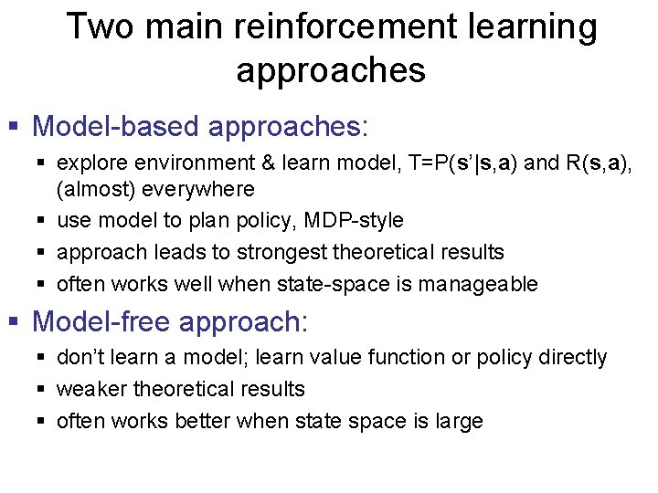
Two main reinforcement learning approaches § Model-based approaches: § explore environment & learn model, T=P(s’|s, a) and R(s, a), (almost) everywhere § use model to plan policy, MDP-style § approach leads to strongest theoretical results § often works well when state-space is manageable § Model-free approach: § don’t learn a model; learn value function or policy directly § weaker theoretical results § often works better when state space is large

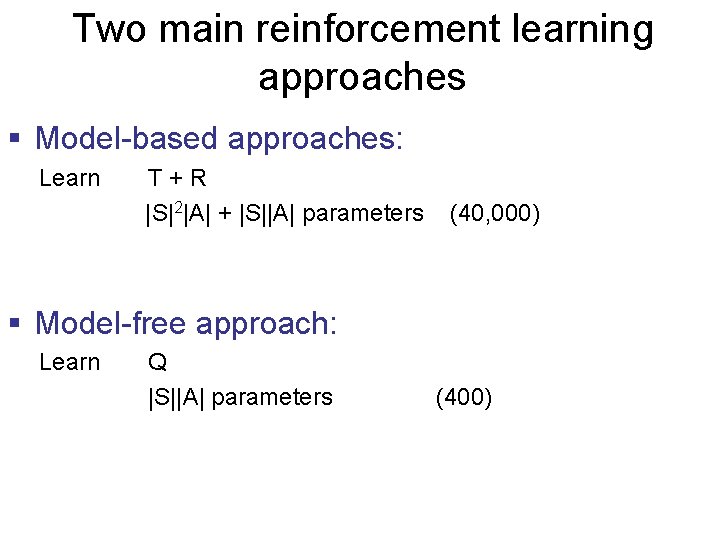
Two main reinforcement learning approaches § Model-based approaches: Learn T+R |S|2|A| + |S||A| parameters (40, 000) § Model-free approach: Learn Q |S||A| parameters (400)

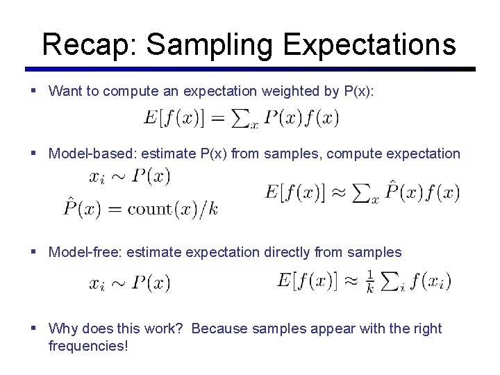
Recap: Sampling Expectations § Want to compute an expectation weighted by P(x): § Model-based: estimate P(x) from samples, compute expectation § Model-free: estimate expectation directly from samples § Why does this work? Because samples appear with the right frequencies!

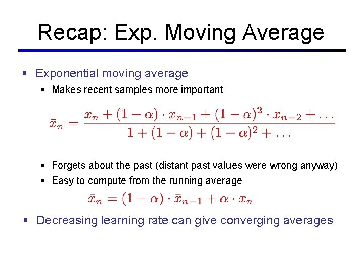
Recap: Exp. Moving Average § Exponential moving average § Makes recent samples more important § Forgets about the past (distant past values were wrong anyway) § Easy to compute from the running average § Decreasing learning rate can give converging averages

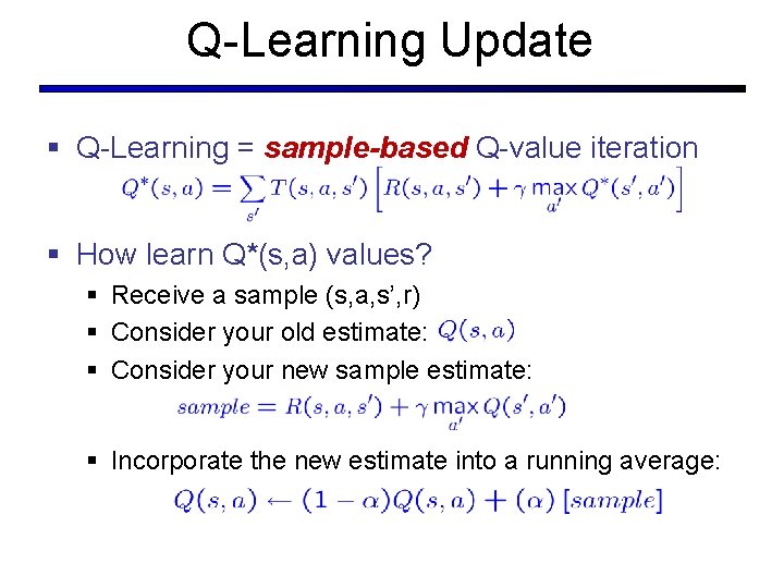
Q-Learning Update § Q-Learning = sample-based Q-value iteration § How learn Q*(s, a) values? § Receive a sample (s, a, s’, r) § Consider your old estimate: § Consider your new sample estimate: § Incorporate the new estimate into a running average:

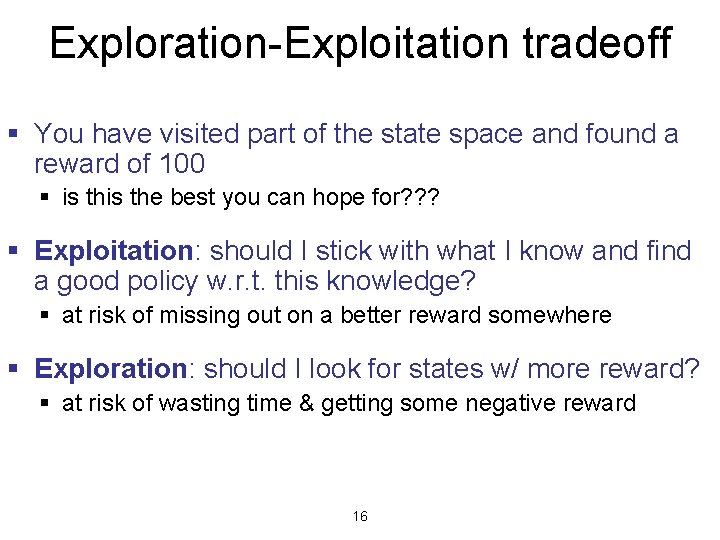
Exploration-Exploitation tradeoff § You have visited part of the state space and found a reward of 100 § is the best you can hope for? ? ? § Exploitation: should I stick with what I know and find a good policy w. r. t. this knowledge? § at risk of missing out on a better reward somewhere § Exploration: should I look for states w/ more reward? § at risk of wasting time & getting some negative reward 16

Exploration / Exploitation § Several schemes for action selection § Simplest: random actions ( greedy) § Every time step, flip a coin § With probability , act randomly § With probability 1 - , act according to current policy § Problems with random actions? § You do explore the space, but keep thrashing around once learning is done § One solution: lower over time § Another solution: exploration functions

Q-Learning: Greedy

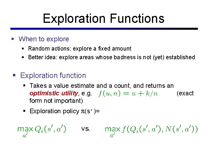
Exploration Functions § When to explore § Random actions: explore a fixed amount § Better idea: explore areas whose badness is not (yet) established § Exploration function § Takes a value estimate and a count, and returns an optimistic utility, e. g. (exact form not important) § Exploration policy π(s’)= vs.

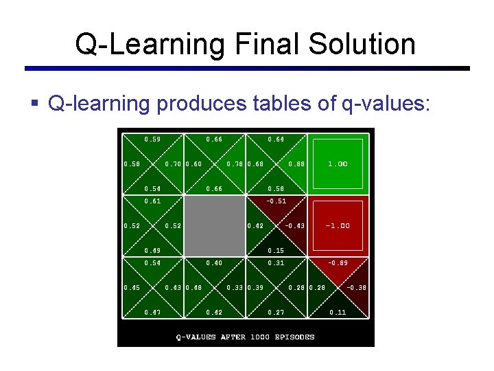
Q-Learning Final Solution § Q-learning produces tables of q-values:

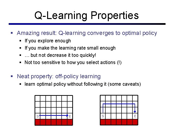
Q-Learning Properties § Amazing result: Q-learning converges to optimal policy § § If you explore enough If you make the learning rate small enough … but not decrease it too quickly! Not too sensitive to how you select actions (!) § Neat property: off-policy learning § learn optimal policy without following it (some caveats) S E

Q-Learning – Small Problem § Doesn’t work § In realistic situations, we can’t possibly learn about every single state! § Too many states to visit them all in training § Too many states to hold the q-tables in memory § Instead, we need to generalize: § Learn about a few states from experience § Generalize that experience to new, similar states (Fundamental idea in machine learning)

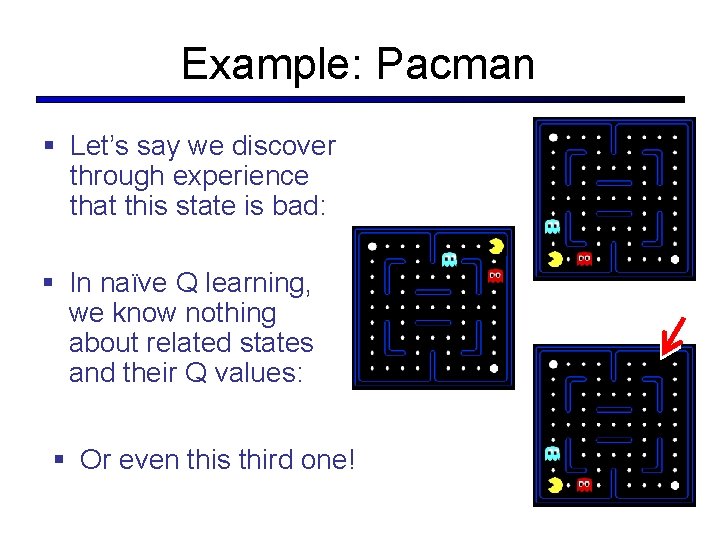
Example: Pacman § Let’s say we discover through experience that this state is bad: § In naïve Q learning, we know nothing about related states and their Q values: § Or even this third one!

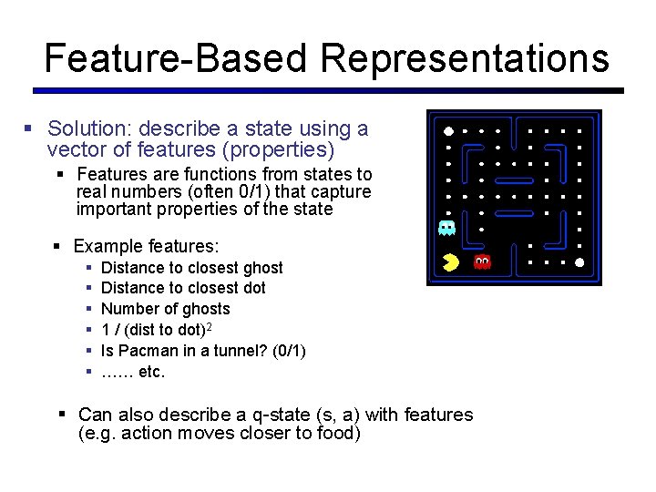
Feature-Based Representations § Solution: describe a state using a vector of features (properties) § Features are functions from states to real numbers (often 0/1) that capture important properties of the state § Example features: § § § Distance to closest ghost Distance to closest dot Number of ghosts 1 / (dist to dot)2 Is Pacman in a tunnel? (0/1) …… etc. § Can also describe a q-state (s, a) with features (e. g. action moves closer to food)

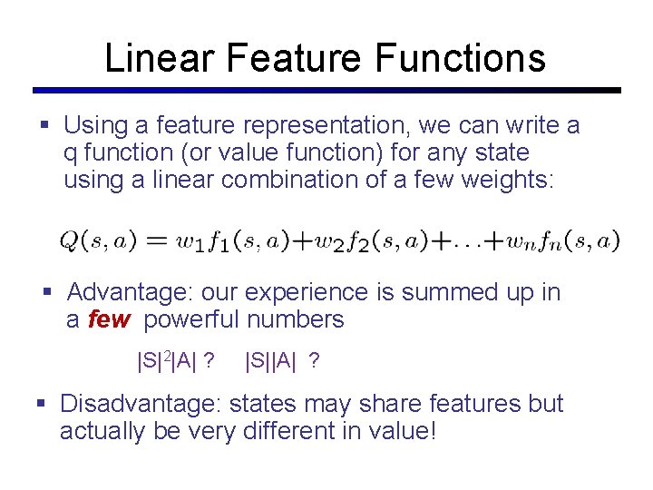
Linear Feature Functions § Using a feature representation, we can write a q function (or value function) for any state using a linear combination of a few weights: § Advantage: our experience is summed up in a few powerful numbers |S|2|A| ? |S||A| ? § Disadvantage: states may share features but actually be very different in value!

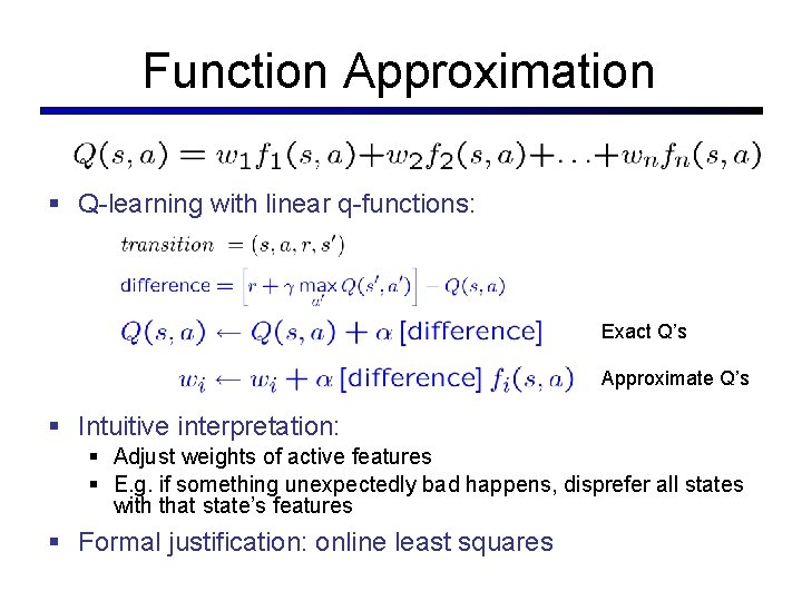
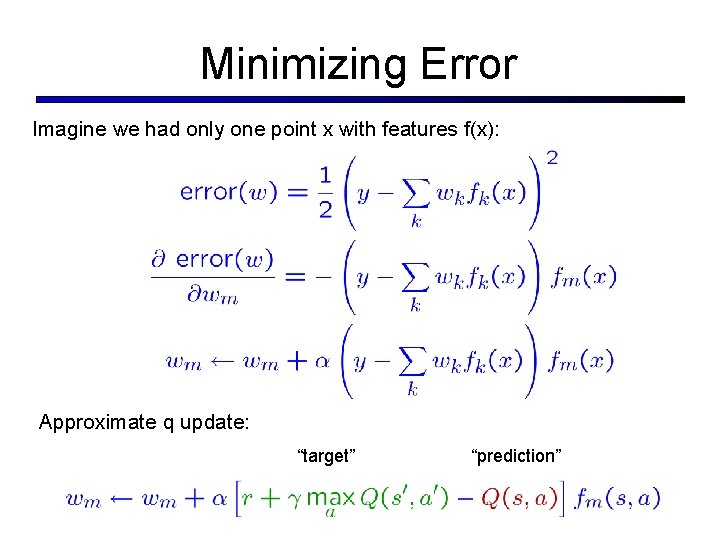
Function Approximation § Q-learning with linear q-functions: Exact Q’s Approximate Q’s § Intuitive interpretation: § Adjust weights of active features § E. g. if something unexpectedly bad happens, disprefer all states with that state’s features § Formal justification: online least squares

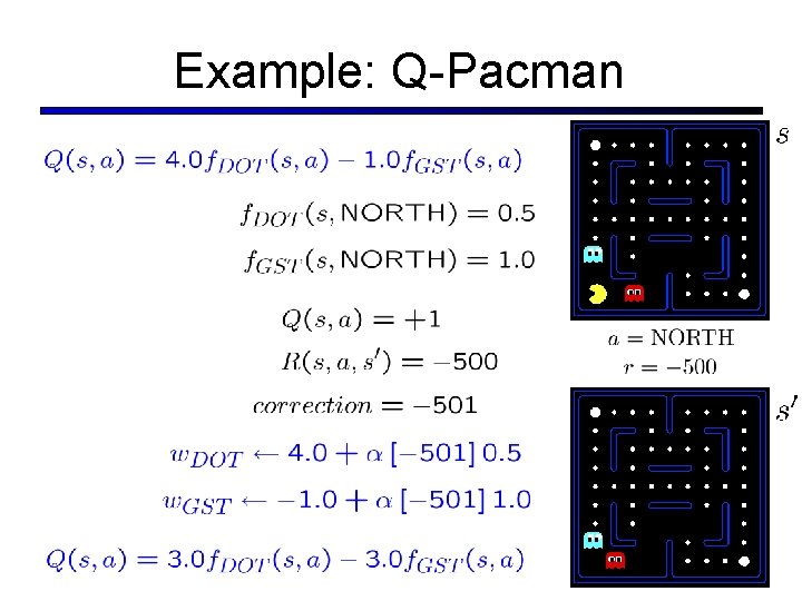
Example: Q-Pacman

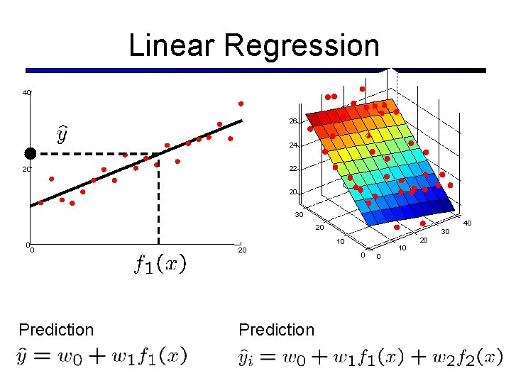
Linear Regression 40 26 24 22 20 20 30 40 20 0 0 Prediction 30 20 10 20 Prediction 0 10 0

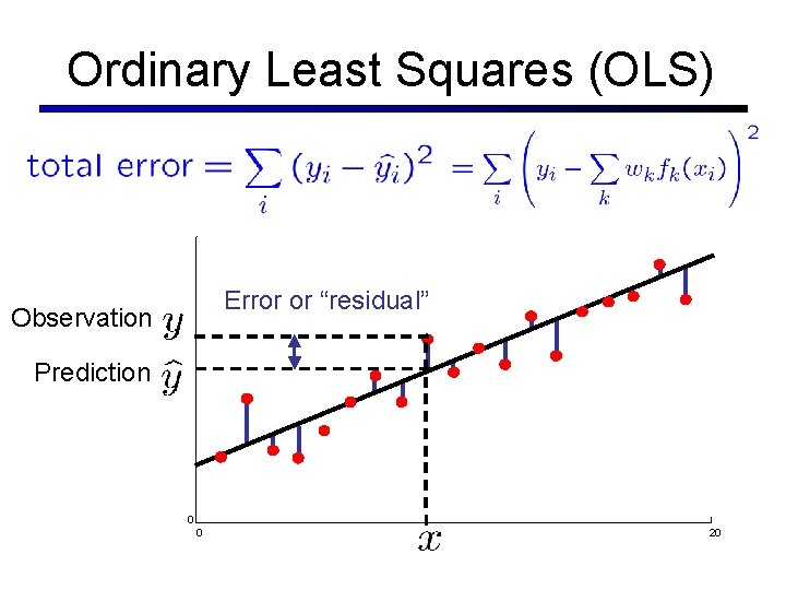
Ordinary Least Squares (OLS) Error or “residual” Observation Prediction 0 0 20

Minimizing Error Imagine we had only one point x with features f(x): Approximate q update: “target” “prediction”

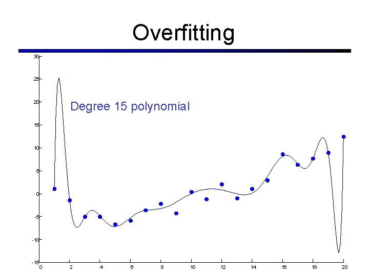
Overfitting 30 25 20 Degree 15 polynomial 15 10 5 0 -5 -10 -15 0 2 4 6 8 10 12 14 16 18 20

Which Algorithm? Q-learning, no features, 50 learning trials:

Which Algorithm? Q-learning, no features, 1000 learning trials:

Which Algorithm? Q-learning, simple features, 50 learning trials:

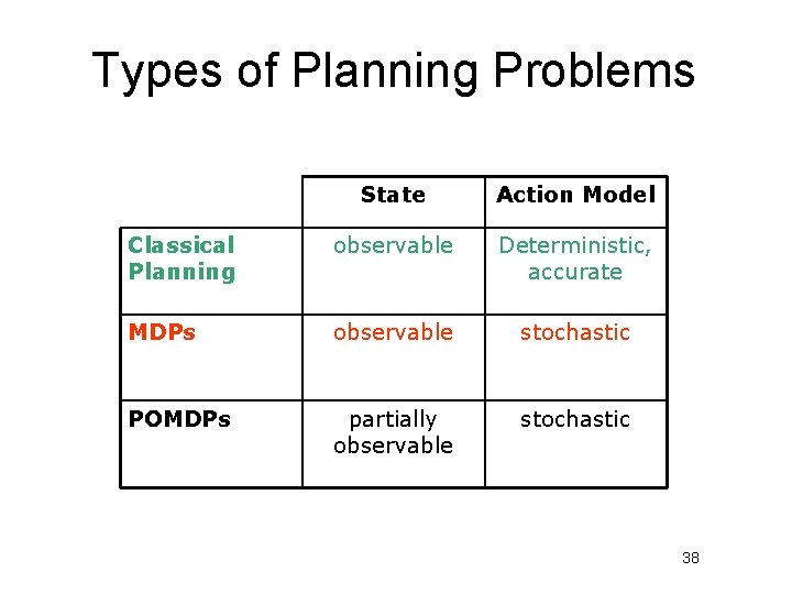
Types of Planning Problems State Action Model Classical Planning observable Deterministic, accurate MDPs observable stochastic POMDPs partially observable stochastic 38

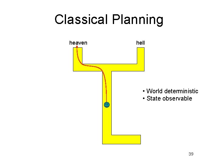
Classical Planning heaven hell • World deterministic • State observable 39

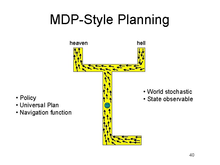
MDP-Style Planning heaven • Policy • Universal Plan • Navigation function hell • World stochastic • State observable 40

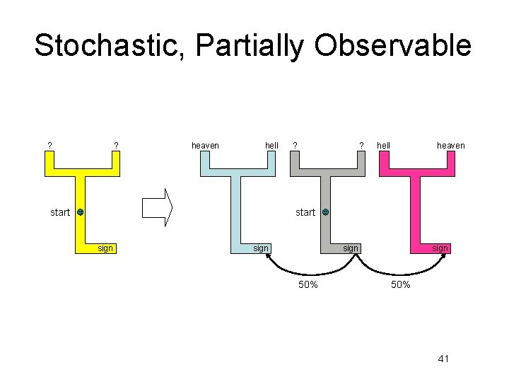
Stochastic, Partially Observable ? ? heaven hell start ? ? hell heaven start sign 50% 41

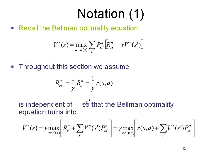
Notation (1) § Recall the Bellman optimality equation: § Throughout this section we assume is independent of so that the Bellman optimality equation turns into 45

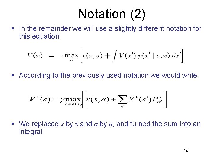
Notation (2) § In the remainder we will use a slightly different notation for this equation: § According to the previously used notation we would write § We replaced s by x and a by u, and turned the sum into an integral. 46

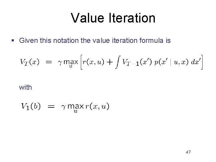
Value Iteration § Given this notation the value iteration formula is with 47

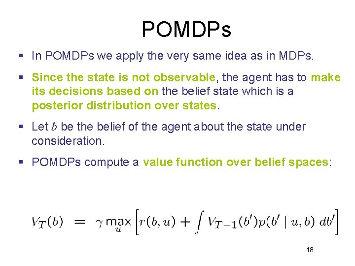
POMDPs § In POMDPs we apply the very same idea as in MDPs. § Since the state is not observable, the agent has to make its decisions based on the belief state which is a posterior distribution over states. § Let b be the belief of the agent about the state under consideration. § POMDPs compute a value function over belief spaces: 48

Problems § Each belief is a probability distribution, thus, each value in a POMDP is a function of an entire probability distribution. § This is problematic, since probability distributions are continuous. § Additionally, we have to deal with the huge complexity of belief spaces. § For finite worlds with finite state, action, and measurement spaces and finite horizons, however, we can effectively represent the value functions by piecewise linear functions. 49

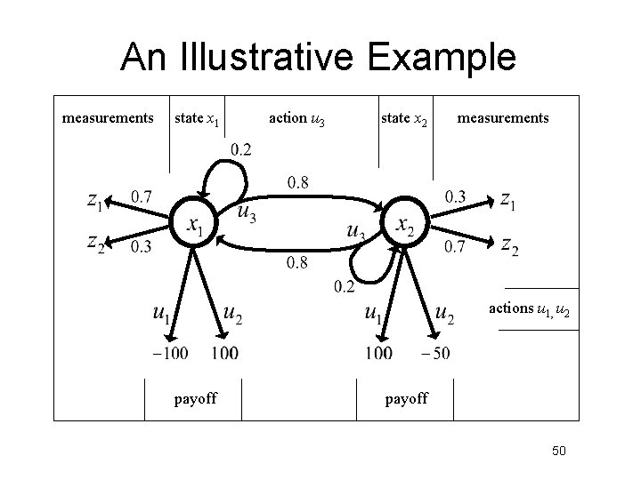
An Illustrative Example measurements state x 1 action u 3 state x 2 measurements actions u 1, u 2 payoff 50

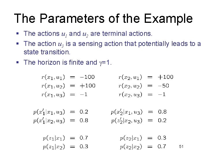
The Parameters of the Example § The actions u 1 and u 2 are terminal actions. § The action u 3 is a sensing action that potentially leads to a state transition. § The horizon is finite and =1. 51

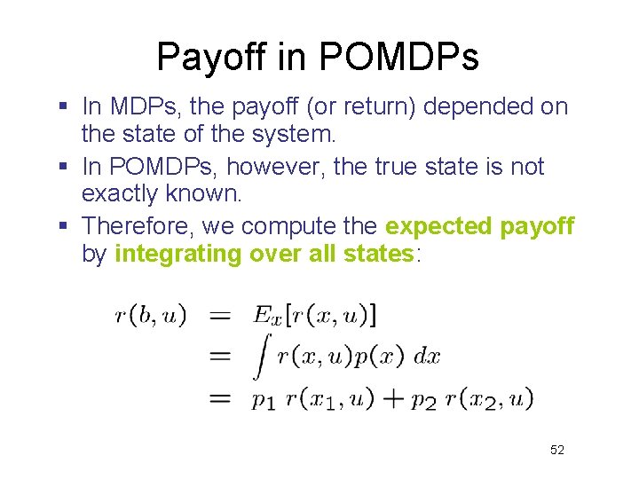
Payoff in POMDPs § In MDPs, the payoff (or return) depended on the state of the system. § In POMDPs, however, the true state is not exactly known. § Therefore, we compute the expected payoff by integrating over all states: 52

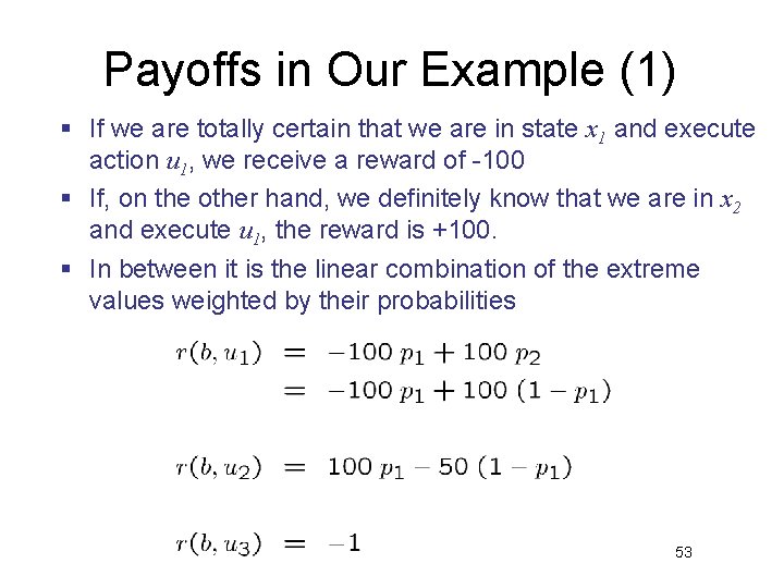
Payoffs in Our Example (1) § If we are totally certain that we are in state x 1 and execute action u 1, we receive a reward of -100 § If, on the other hand, we definitely know that we are in x 2 and execute u 1, the reward is +100. § In between it is the linear combination of the extreme values weighted by their probabilities 53

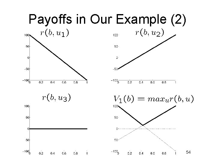
Payoffs in Our Example (2) 54

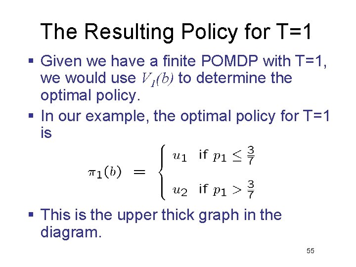
The Resulting Policy for T=1 § Given we have a finite POMDP with T=1, we would use V 1(b) to determine the optimal policy. § In our example, the optimal policy for T=1 is § This is the upper thick graph in the diagram. 55

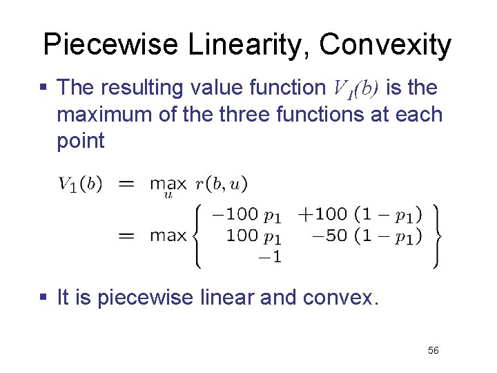
Piecewise Linearity, Convexity § The resulting value function V 1(b) is the maximum of the three functions at each point § It is piecewise linear and convex. 56

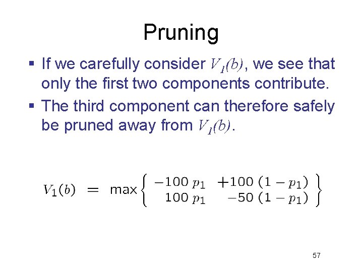
Pruning § If we carefully consider V 1(b), we see that only the first two components contribute. § The third component can therefore safely be pruned away from V 1(b). 57

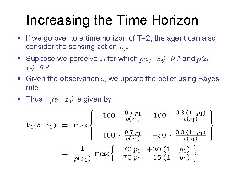
Increasing the Time Horizon § If we go over to a time horizon of T=2, the agent can also consider the sensing action u 3. § Suppose we perceive z 1 for which p(z 1 | x 1)=0. 7 and p(z 1| x 2)=0. 3. § Given the observation z 1 we update the belief using Bayes rule. § Thus V 1(b | z 1) is given by 58

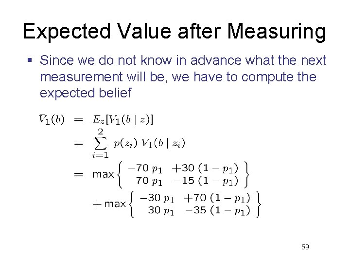
Expected Value after Measuring § Since we do not know in advance what the next measurement will be, we have to compute the expected belief 59

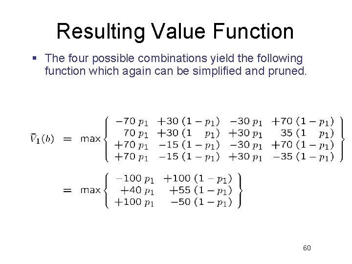
Resulting Value Function § The four possible combinations yield the following function which again can be simplified and pruned. 60

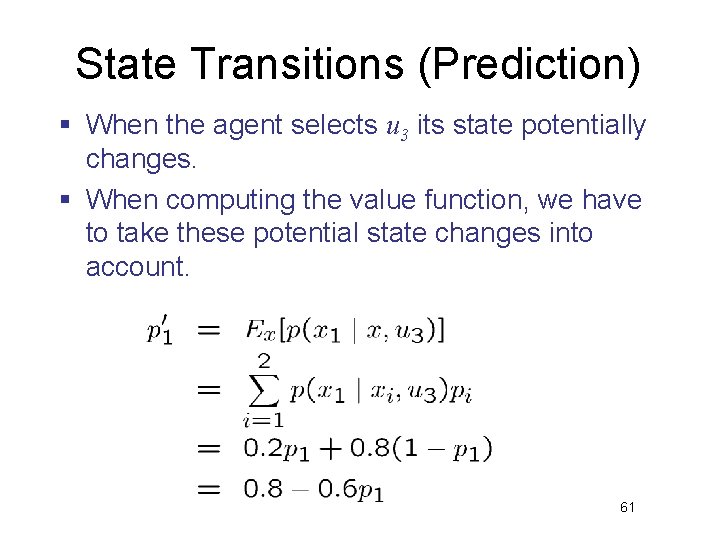
State Transitions (Prediction) § When the agent selects u 3 its state potentially changes. § When computing the value function, we have to take these potential state changes into account. 61

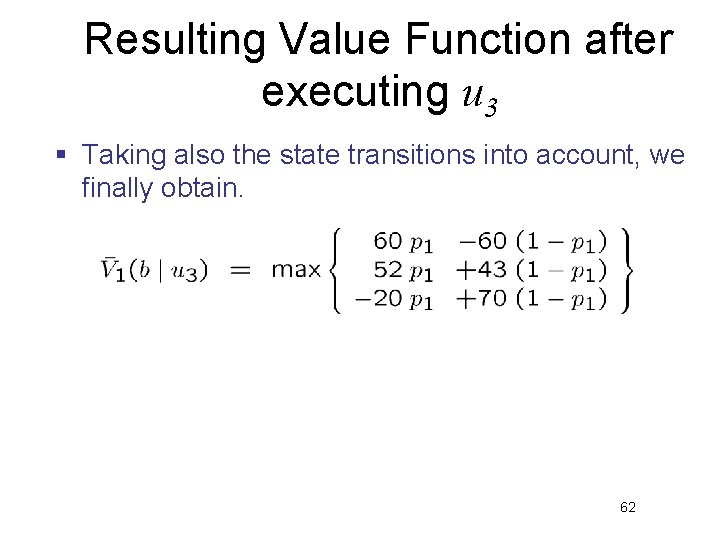
Resulting Value Function after executing u 3 § Taking also the state transitions into account, we finally obtain. 62

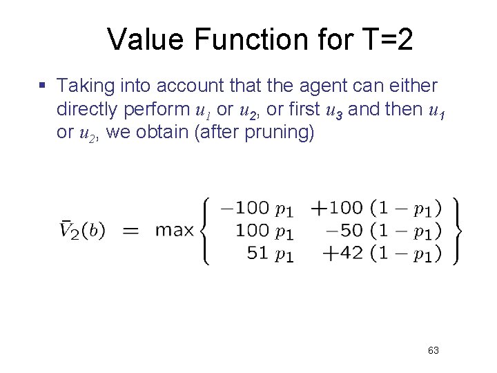
Value Function for T=2 § Taking into account that the agent can either directly perform u 1 or u 2, or first u 3 and then u 1 or u 2, we obtain (after pruning) 63

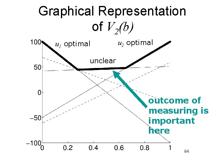
Graphical Representation of V 2(b) u 1 optimal u 2 optimal unclear outcome of measuring is important here 64

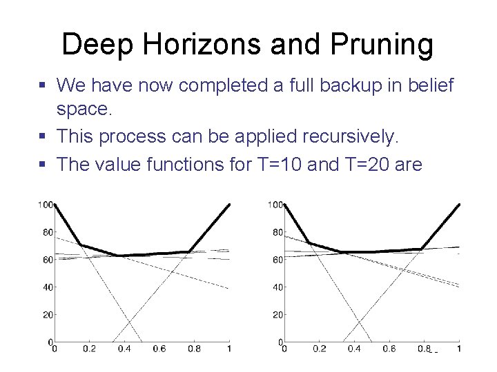
Deep Horizons and Pruning § We have now completed a full backup in belief space. § This process can be applied recursively. § The value functions for T=10 and T=20 are 65

Why Pruning is Essential § Each update introduces additional linear components to V. § Each measurement squares the number of linear components. § Thus, an unpruned value function for T=20 includes more than 10547, 864 linear functions. § At T=30 we have 10561, 012, 337 linear functions. § The pruned value functions at T=20, in comparison, contains only 12 linear components. § The combinatorial explosion of linear components in the value function are the major reason why POMDPs are impractical for most applications. 66

A Summary on POMDPs § POMDPs compute the optimal action in partially observable, stochastic domains. § For finite horizon problems, the resulting value functions are piecewise linear and convex. § In each iteration the number of linear constraints grows exponentially. § POMDPs so far have only been applied successfully to very small state spaces with small numbers of possible observations and actions. 67