CSE 421 Algorithms Richard Anderson Lecture 14 Inversions

Divide and Conquer Algorithms • • • Mergesort, Quicksort Strassen’s Algorithm Closest Pair Algorithm

Inversion Problem • Let a 1, . . . an be a permutation of

Counting Inversions 11 12 4 1 7 2 3 15 9 5 16 8

Count the Inversions 4 2 11 12 4 1 7 3 2 3 15

Problem – how do we count inversions between sub problems in O(n) time? •

Use the merge algorithm to count inversions 1 4 11 12 5 8 9

Inversions • Counting inversions between two sorted lists – O(1) per element to count

Integer Arithmetic 9715480283945084383094856701043643845790217965702956767 + 1242431098234099057329075097179898430928779579277597977 Runtime for standard algorithm to add two n digit

Recursive Algorithm (First attempt) x = x 1 2 n/2 + x 0 y

Simple algebra x = x 1 2 n/2 + x 0 y = y

Karatsuba’s Algorithm Multiply n-digit integers x and y Let x = x 1 2

FFT, Convolution and Polynomial Multiplication • Preview – FFT - O(n log n) algorithm

Complex Analysis • • • Polar coordinates: reqi = cos q + i sin

Convolution • a 0, a 1, a 2, . . . , am-1 •

Applications of Convolution • Polynomial Multiplication • Signal processing – Gaussian smoothing – Sequence

FFT Overview • Polynomial interpolation – Given n+1 points (xi, yi), there is a

Polynomial Multiplication n-1 degree polynomials A(x) = a 0 + a 1 x +

FFT • Polynomial A(x) = a 0 + a 1 x +. . .

Slides: 20

Download presentation

CSE 421 Algorithms Richard Anderson Lecture 14 Inversions, Multiplication, FFT

Divide and Conquer Algorithms • • • Mergesort, Quicksort Strassen’s Algorithm Closest Pair Algorithm (2 d) Inversion counting Integer Multiplication (Karatsuba’s Algorithm) FFT – Polynomial Multiplication – Convolution

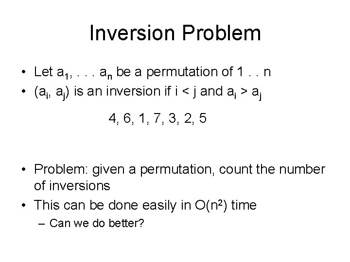
Inversion Problem • Let a 1, . . . an be a permutation of 1. . n • (ai, aj) is an inversion if i < j and ai > aj 4, 6, 1, 7, 3, 2, 5 • Problem: given a permutation, count the number of inversions • This can be done easily in O(n 2) time – Can we do better?

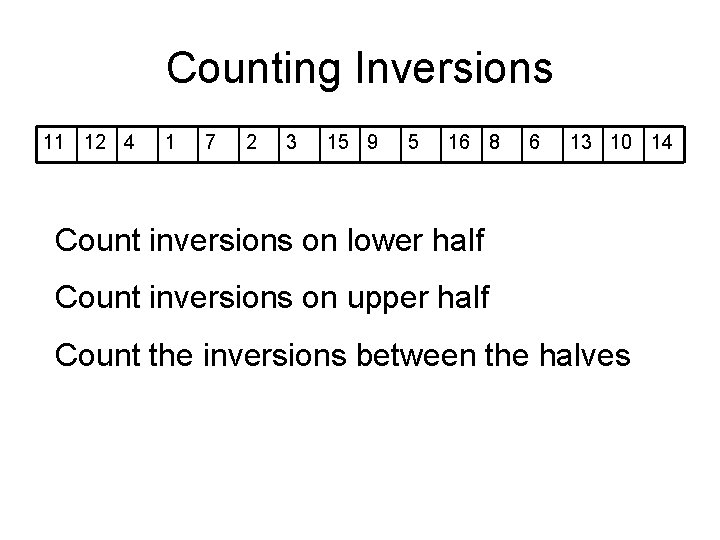
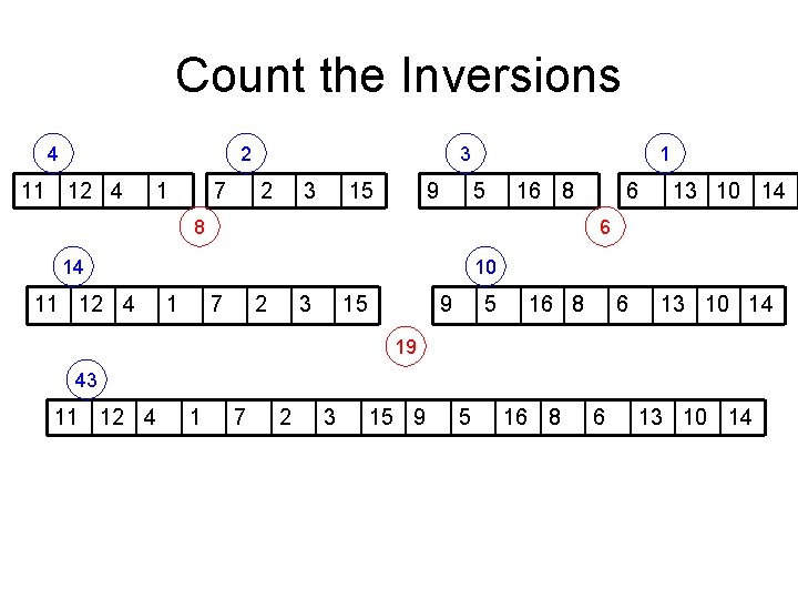
Counting Inversions 11 12 4 1 7 2 3 15 9 5 16 8 6 13 10 14 Count inversions on lower half Count inversions on upper half Count the inversions between the halves

Count the Inversions 4 2 11 12 4 1 7 3 2 3 15 9 1 5 16 8 8 13 10 14 6 14 11 12 4 6 10 1 7 2 3 15 9 5 16 8 6 13 10 14 19 43 11 12 4 1 7 2 3 15 9 5 16 8 6 13 10 14

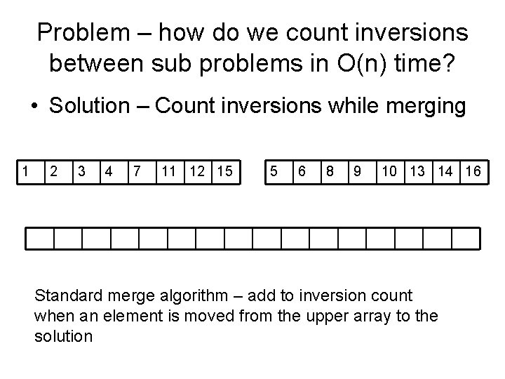
Problem – how do we count inversions between sub problems in O(n) time? • Solution – Count inversions while merging 1 2 3 4 7 11 12 15 5 6 8 9 10 13 14 16 Standard merge algorithm – add to inversion count when an element is moved from the upper array to the solution

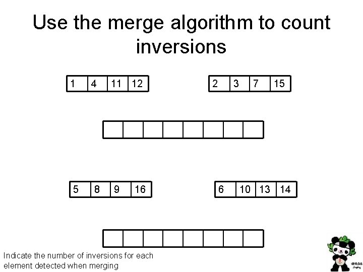
Use the merge algorithm to count inversions 1 4 11 12 5 8 9 16 Indicate the number of inversions for each element detected when merging 2 3 6 7 15 10 13 14

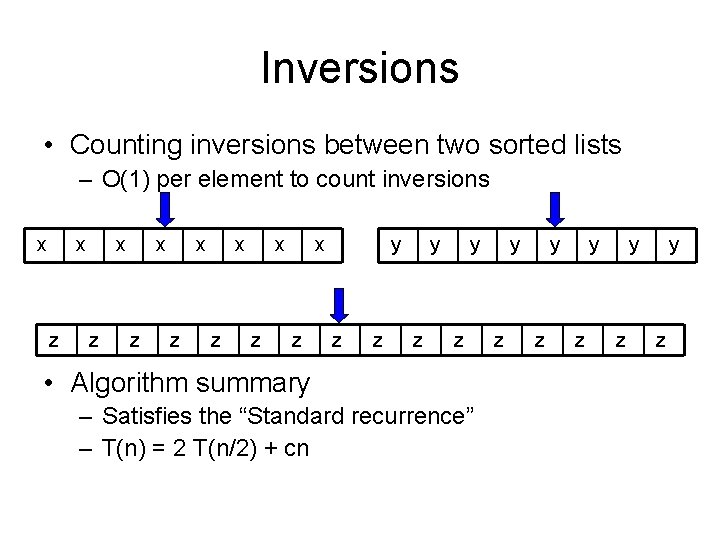
Inversions • Counting inversions between two sorted lists – O(1) per element to count inversions x x z x z y z y z • Algorithm summary – Satisfies the “Standard recurrence” – T(n) = 2 T(n/2) + cn y z y z y z

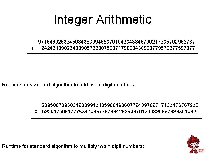
Integer Arithmetic 9715480283945084383094856701043643845790217965702956767 + 1242431098234099057329075097179898430928779579277597977 Runtime for standard algorithm to add two n digit numbers: 2095067093034680994318596846868779409766717133476767930 X 5920175091777634709677679342929097012308956679993010921 Runtime for standard algorithm to multiply two n digit numbers:

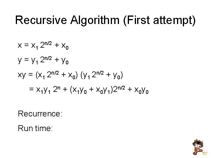
Recursive Algorithm (First attempt) x = x 1 2 n/2 + x 0 y = y 1 2 n/2 + y 0 xy = (x 1 2 n/2 + x 0) (y 1 2 n/2 + y 0) = x 1 y 1 2 n + (x 1 y 0 + x 0 y 1)2 n/2 + x 0 y 0 Recurrence: Run time:

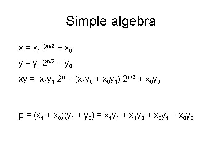
Simple algebra x = x 1 2 n/2 + x 0 y = y 1 2 n/2 + y 0 xy = x 1 y 1 2 n + (x 1 y 0 + x 0 y 1) 2 n/2 + x 0 y 0 p = (x 1 + x 0)(y 1 + y 0) = x 1 y 1 + x 1 y 0 + x 0 y 1 + x 0 y 0

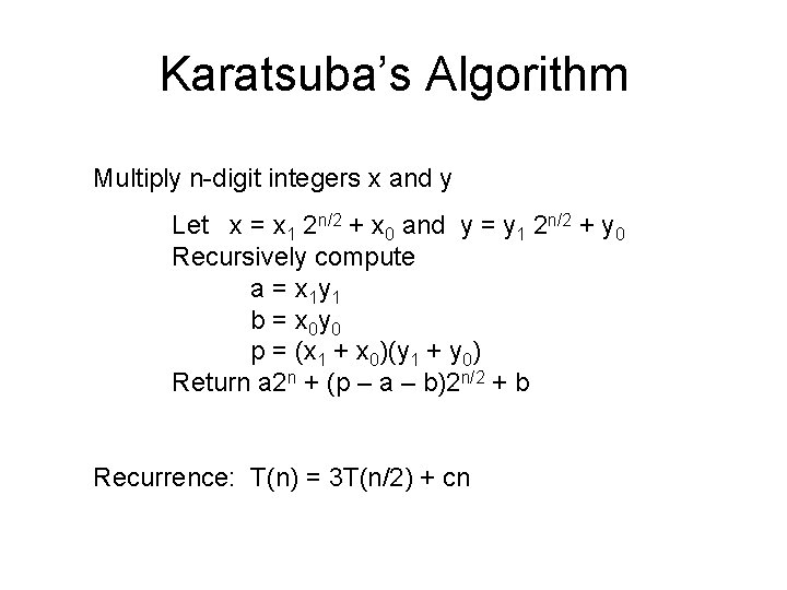
Karatsuba’s Algorithm Multiply n-digit integers x and y Let x = x 1 2 n/2 + x 0 and y = y 1 2 n/2 + y 0 Recursively compute a = x 1 y 1 b = x 0 y 0 p = (x 1 + x 0)(y 1 + y 0) Return a 2 n + (p – a – b)2 n/2 + b Recurrence: T(n) = 3 T(n/2) + cn

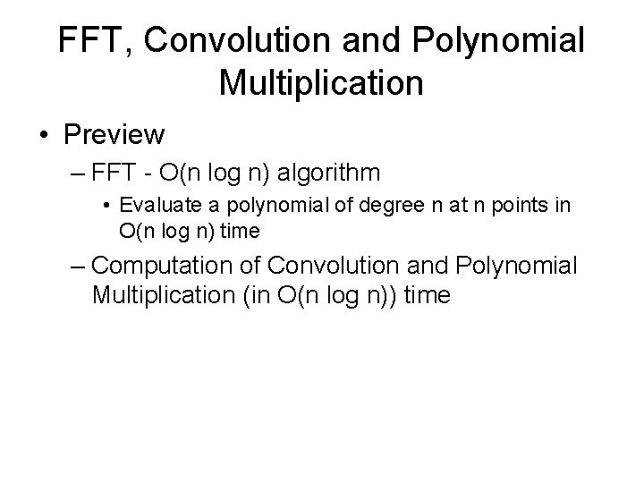
FFT, Convolution and Polynomial Multiplication • Preview – FFT - O(n log n) algorithm • Evaluate a polynomial of degree n at n points in O(n log n) time – Computation of Convolution and Polynomial Multiplication (in O(n log n)) time

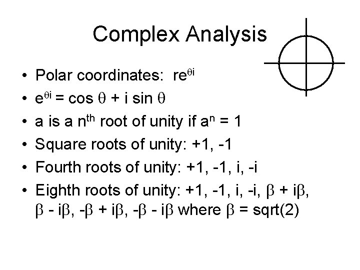
Complex Analysis • • • Polar coordinates: reqi = cos q + i sin q a is a nth root of unity if an = 1 Square roots of unity: +1, -1 Fourth roots of unity: +1, -1, i, -i Eighth roots of unity: +1, -1, i, -i, b + ib, b - ib, -b + ib, -b - ib where b = sqrt(2)

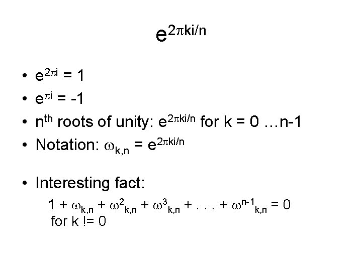
e 2 pki/n • • e 2 pi = 1 epi = -1 nth roots of unity: e 2 pki/n for k = 0 …n-1 Notation: wk, n = e 2 pki/n • Interesting fact: 1 + wk, n + w 2 k, n + w 3 k, n +. . . + wn-1 k, n = 0 for k != 0

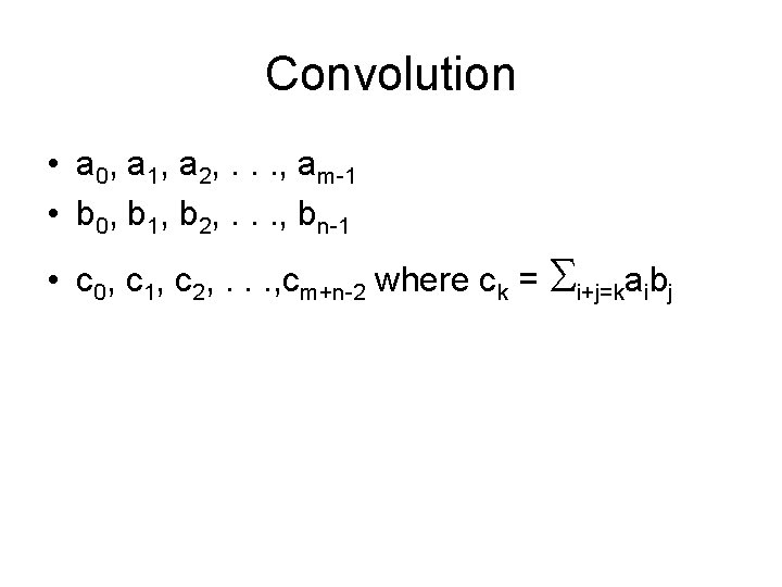
Convolution • a 0, a 1, a 2, . . . , am-1 • b 0, b 1, b 2, . . . , bn-1 • c 0, c 1, c 2, . . . , cm+n-2 where ck = Si+j=kaibj

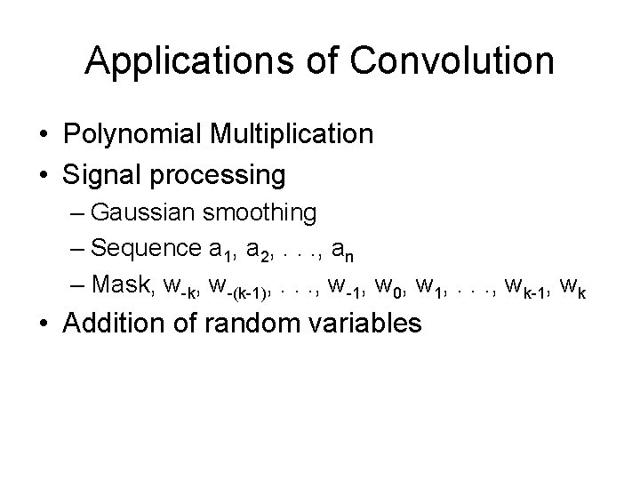
Applications of Convolution • Polynomial Multiplication • Signal processing – Gaussian smoothing – Sequence a 1, a 2, . . . , an – Mask, w-(k-1), . . . , w-1, w 0, w 1, . . . , wk-1, wk • Addition of random variables

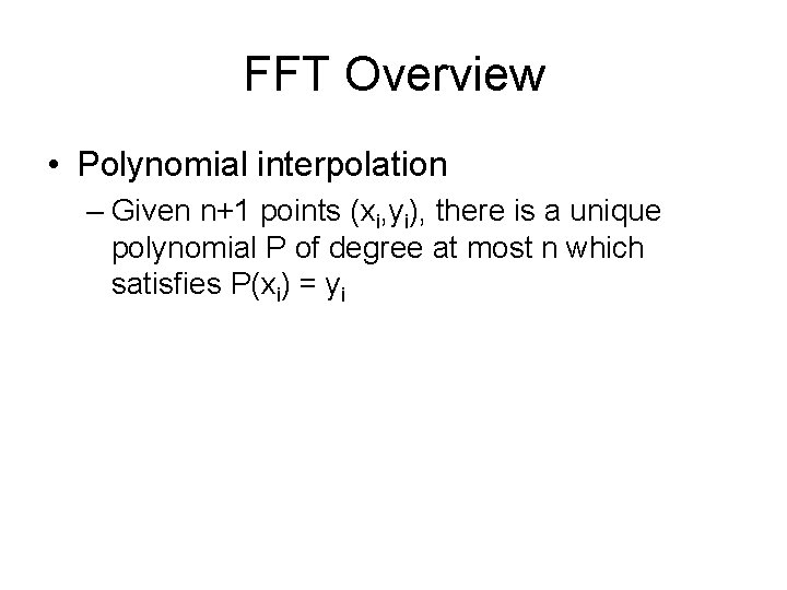
FFT Overview • Polynomial interpolation – Given n+1 points (xi, yi), there is a unique polynomial P of degree at most n which satisfies P(xi) = yi

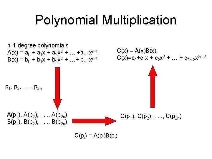
Polynomial Multiplication n-1 degree polynomials A(x) = a 0 + a 1 x + a 2 x 2 + … +an-1 xn-1, B(x) = b 0 + b 1 x + b 2 x 2 + …+ bn-1 xn-1 C(x) = A(x)B(x) C(x)=c 0+c 1 x + c 2 x 2 + … + c 2 n-2 x 2 n-2 p 1, p 2, . . . , p 2 n A(p 1), A(p 2), . . . , A(p 2 n) B(p 1), B(p 2), . . . , B(p 2 n) C(p 1), C(p 2), . . . , C(p 2 n) C(pi) = A(pi)B(pi)

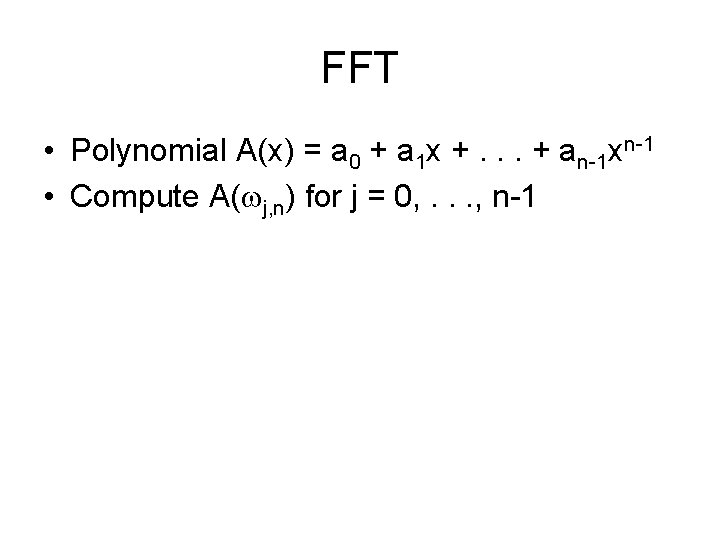
FFT • Polynomial A(x) = a 0 + a 1 x +. . . + an-1 xn-1 • Compute A(wj, n) for j = 0, . . . , n-1