CSE 416 DIGITAL CONTROL Lecture 03 State Variable

CSE 416: DIGITAL CONTROL Lecture 03: State Variable Models Dr. Ahmed Mahmoud, 9/11/2020

History of State Variable Models • Rudolf Emil Kalman (1930– 2016) was a Hungarian-American electrical engineer, mathematician, and inventor. • In late 1950 s, Kalman introduced modern control theory, which employs matrix-vector differential equations and uses the calculus of variations to generate optimal control policies for these systems (Kalman, 1963). • One important result is that for a linear system with a quadratic performance index the optimal control policy is a simple linear combination of the matrix-vector differential equation variables or states. • In early 1960 s, Kalman (1960) introduced the concept of optimal state estimation when the system has random disturbances, and the measurements of system outputs are contaminated by additive noise. 9/11/2019 CSE 416: Digital Control, Lec 03 2

Terms of State Variable Model 9/11/2019 CSE 416: Digital Control, Lec 03 3

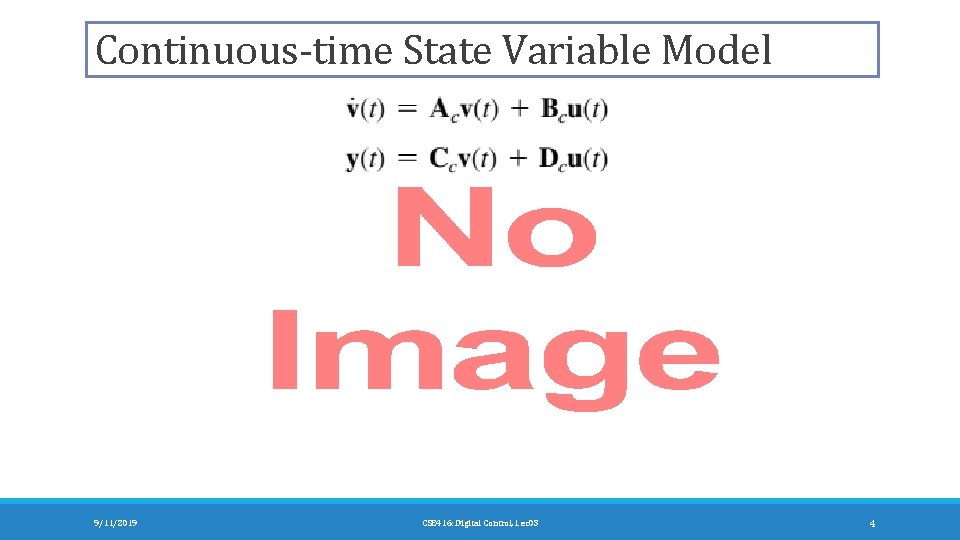
Continuous-time State Variable Model 9/11/2019 CSE 416: Digital Control, Lec 03 4

Example of Continuous-time State Variable Model • The system equations are: • Choose the state variables as: • The state variable model is: 9/11/2019 CSE 416: Digital Control, Lec 03 5

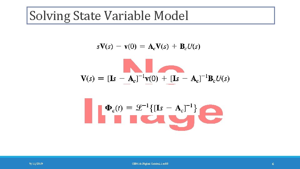
Solving State Variable Model 9/11/2019 CSE 416: Digital Control, Lec 03 6

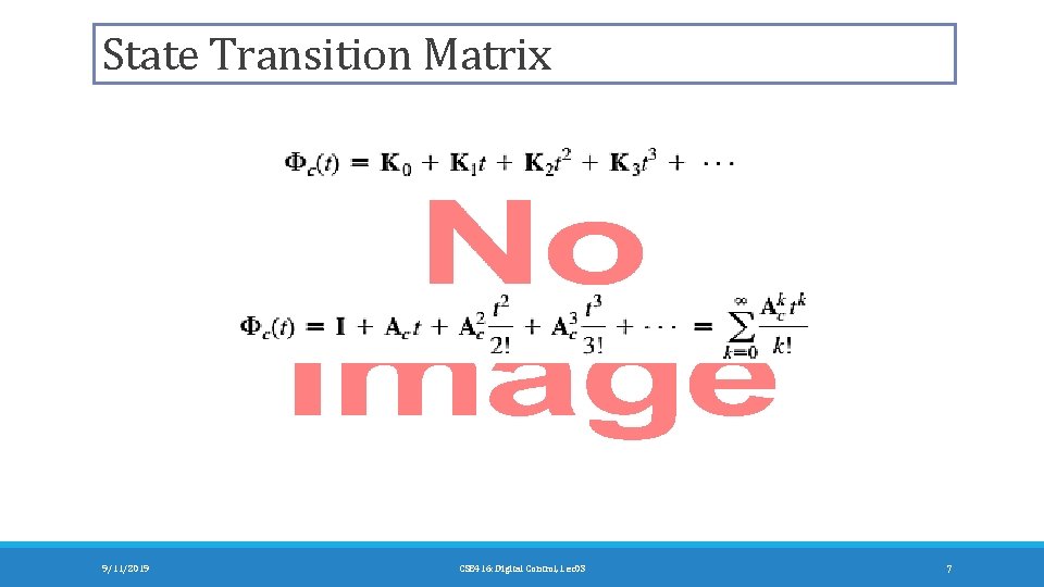
State Transition Matrix 9/11/2019 CSE 416: Digital Control, Lec 03 7

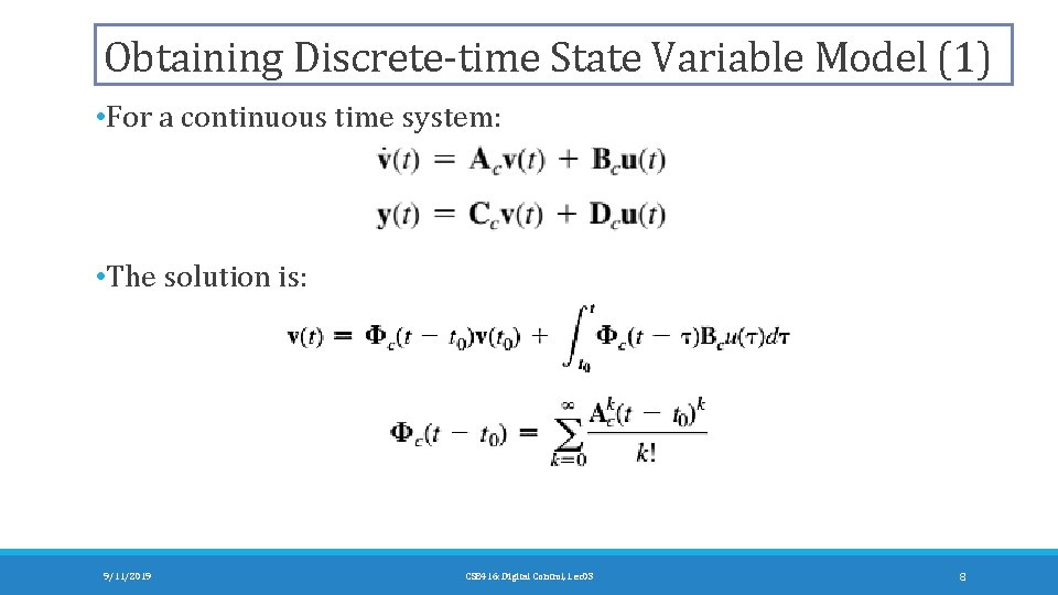
Obtaining Discrete-time State Variable Model (1) • For a continuous time system: • The solution is: 9/11/2019 CSE 416: Digital Control, Lec 03 8

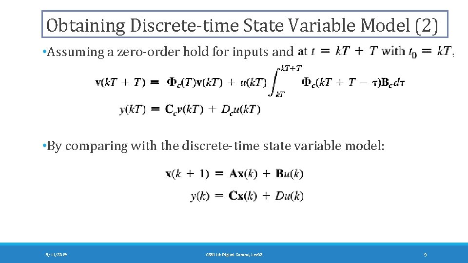
Obtaining Discrete-time State Variable Model (2) • Assuming a zero-order hold for inputs and • By comparing with the discrete-time state variable model: 9/11/2019 CSE 416: Digital Control, Lec 03 9

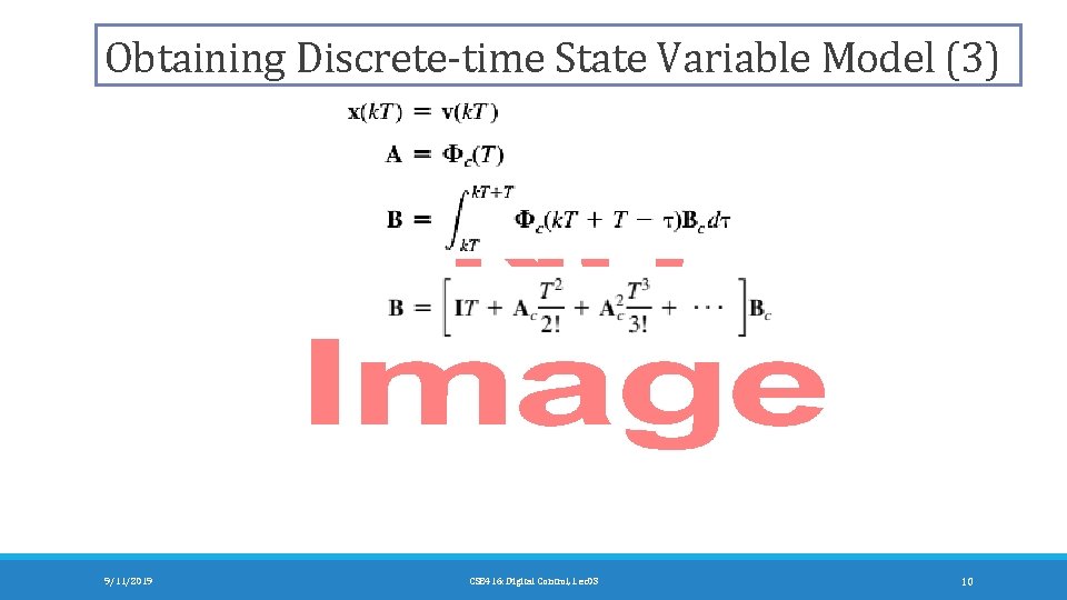
Obtaining Discrete-time State Variable Model (3) 9/11/2019 CSE 416: Digital Control, Lec 03 10

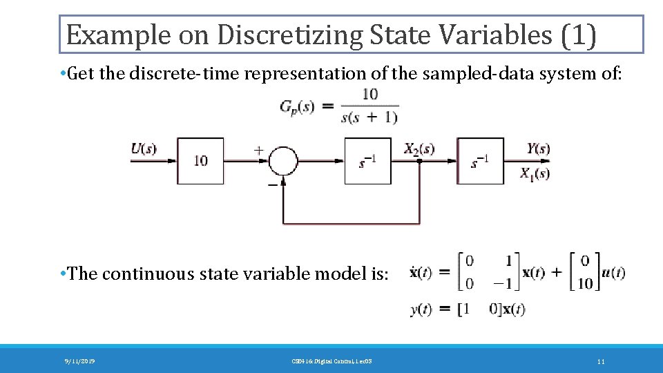
Example on Discretizing State Variables (1) • Get the discrete-time representation of the sampled-data system of: • The continuous state variable model is: 9/11/2019 CSE 416: Digital Control, Lec 03 11

Example on Discretizing State Variables (2) 9/11/2019 CSE 416: Digital Control, Lec 03 12

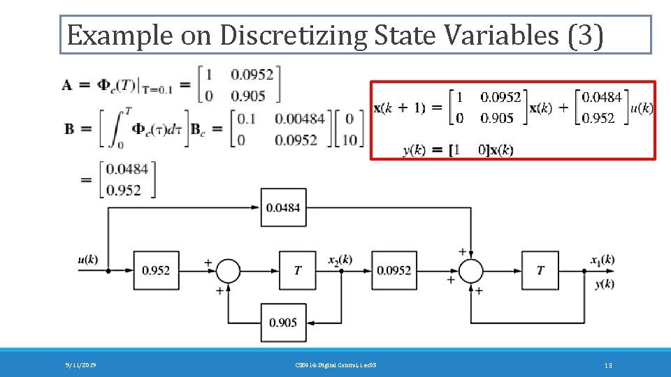
Example on Discretizing State Variables (3) 9/11/2019 CSE 416: Digital Control, Lec 03 13

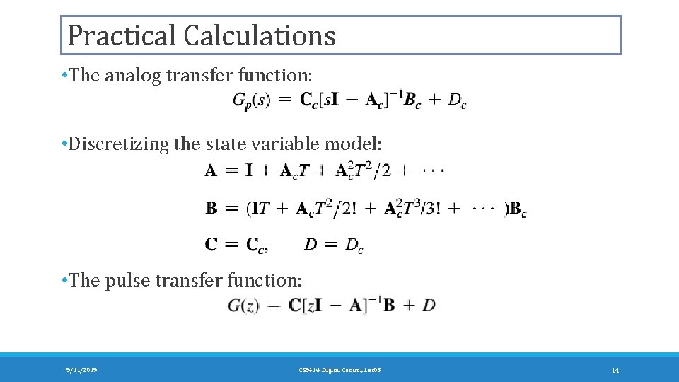
Practical Calculations • The analog transfer function: • Discretizing the state variable model: • The pulse transfer function: 9/11/2019 CSE 416: Digital Control, Lec 03 14

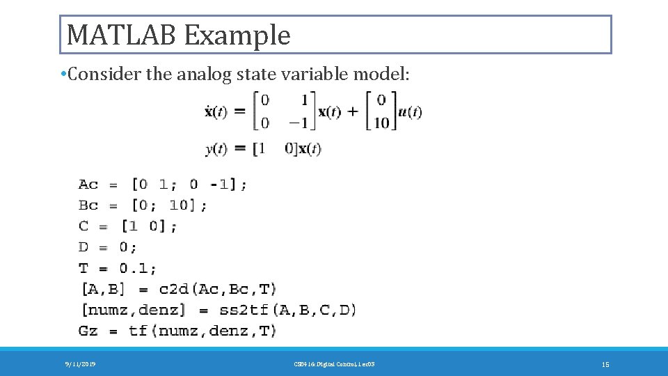
MATLAB Example • Consider the analog state variable model: 9/11/2019 CSE 416: Digital Control, Lec 03 15

Canonical Forms • Any system has one unique transfer function representation. • Converting a state-space realization to a transfer function form may lose some internal information about the system, and may provide a description of a system which is stable, when the state-space realization is unstable at certain points. • Various canonical state variable models can be derived from the above transfer function model. 9/11/2019 CSE 416: Digital Control, Lec 03 16

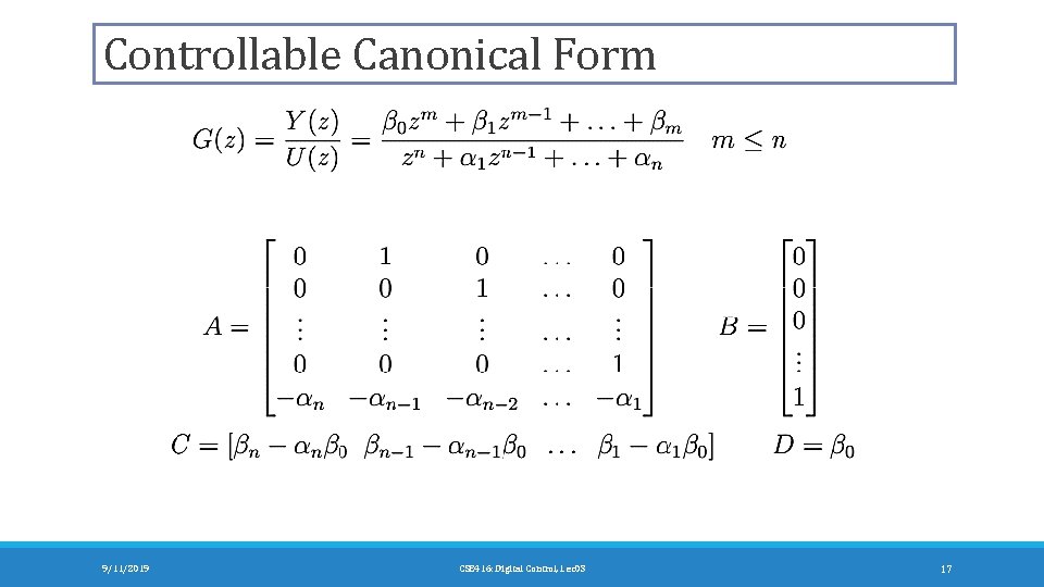
Controllable Canonical Form 9/11/2019 CSE 416: Digital Control, Lec 03 17

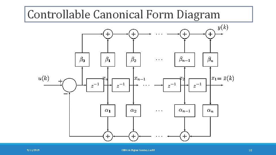
Controllable Canonical Form Diagram 9/11/2019 CSE 416: Digital Control, Lec 03 18

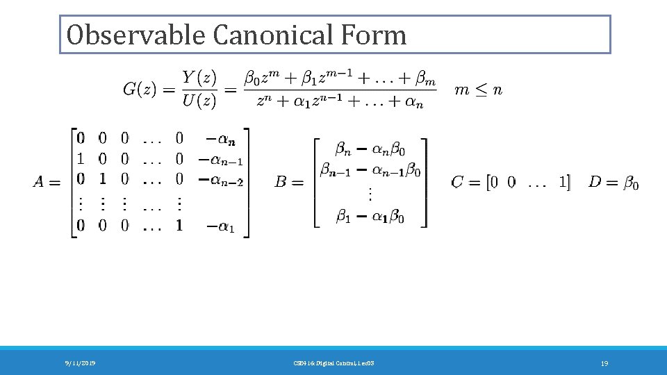
Observable Canonical Form 9/11/2019 CSE 416: Digital Control, Lec 03 19

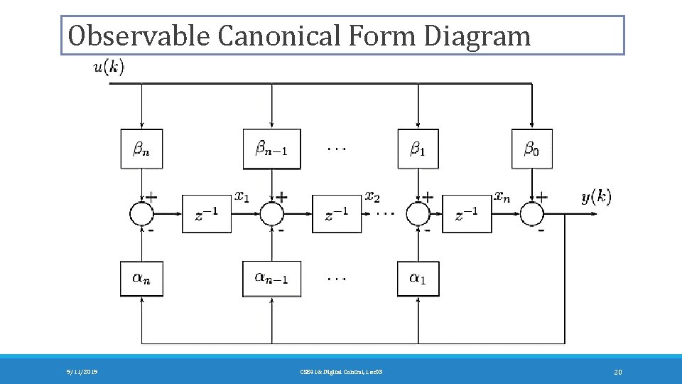
Observable Canonical Form Diagram 9/11/2019 CSE 416: Digital Control, Lec 03 20

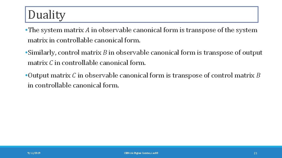
Duality • The system matrix A in observable canonical form is transpose of the system matrix in controllable canonical form. • Similarly, control matrix B in observable canonical form is transpose of output matrix C in controllable canonical form. • Output matrix C in observable canonical form is transpose of control matrix B in controllable canonical form. 9/11/2019 CSE 416: Digital Control, Lec 03 21

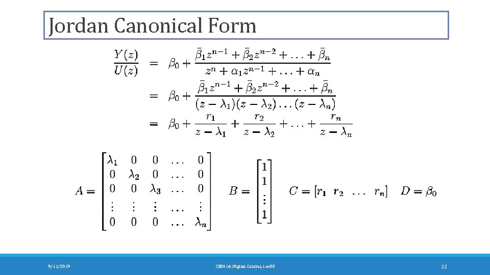
Jordan Canonical Form 9/11/2019 CSE 416: Digital Control, Lec 03 22

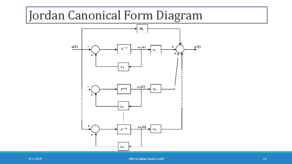
Jordan Canonical Form Diagram 9/11/2019 CSE 416: Digital Control, Lec 03 23

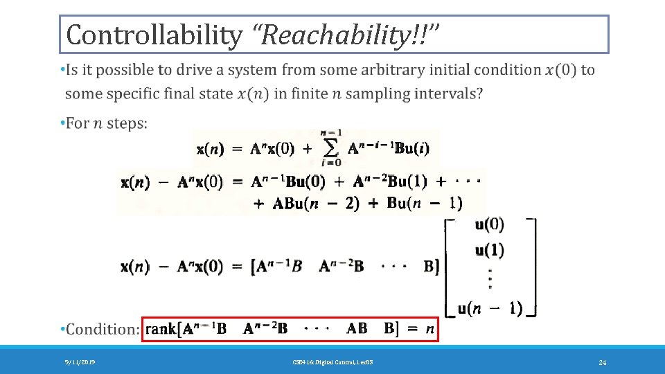
Controllability “Reachability!!” 9/11/2019 CSE 416: Digital Control, Lec 03 24

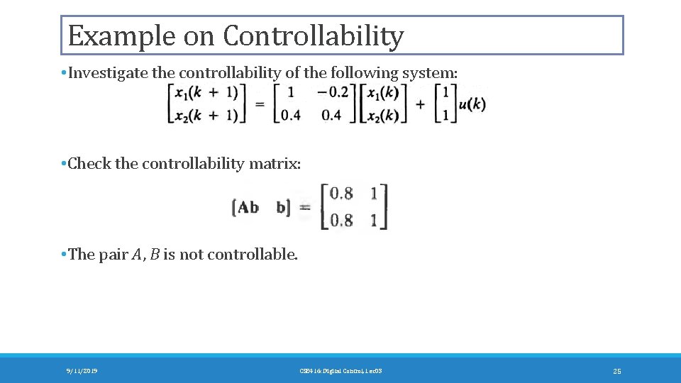
Example on Controllability • Investigate the controllability of the following system: • Check the controllability matrix: • The pair A, B is not controllable. 9/11/2019 CSE 416: Digital Control, Lec 03 25

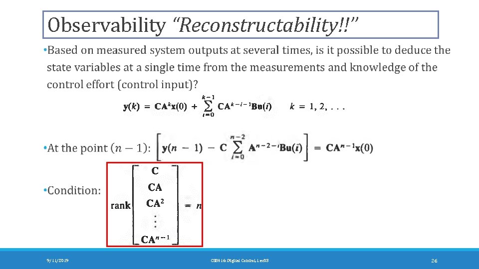
Observability “Reconstructability!!” 9/11/2019 CSE 416: Digital Control, Lec 03 26

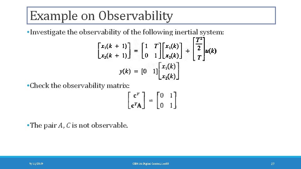
Example on Observability • Investigate the observability of the following inertial system: • Check the observability matrix: • The pair A, C is not observable. 9/11/2019 CSE 416: Digital Control, Lec 03 27

Reading • Read Sections 2. 9 to 2. 12. • Read Sections 4. 8 to 4. 11. 9/11/2019 CSE 416: Digital Control, Lec 03 28