CSE 410 Computer Graphics Sessional Virtual Realism TEXTURE

CSE 410 Computer Graphics Sessional Virtual Realism TEXTURE MAPPING

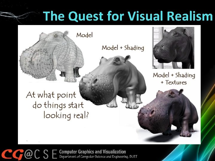
The Quest for Visual Realism

Why Texture Map? �So far we have done flat shading and Gouraud/Phong shading �Not good to represent everything in real world �What are some of our other options? �Represent everything with tiny polygons � Geometry would get complicated very quickly �Apply textures across the polygons �This allows for less geometry but the image looks almost as good

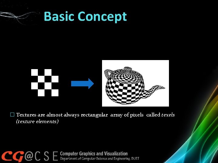
• • Basic Concept Pasting an image onto a model An image is mapped onto the 2 D domain of a 3 D model � Textures are almost always rectangular array of pixels called texels (texture elements)

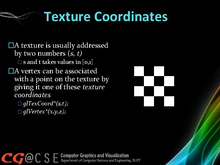
Texture Coordinates �A texture is usually addressed by two numbers (s, t) � s and t takes values in [0, 1] �A vertex can be associated with a point on the texture by giving it one of these texture coordinates [0, 1] t � gl. Tex. Coord*(s, t); � gl. Vertex*(x, y, z); [0, 0] s [1, 0]

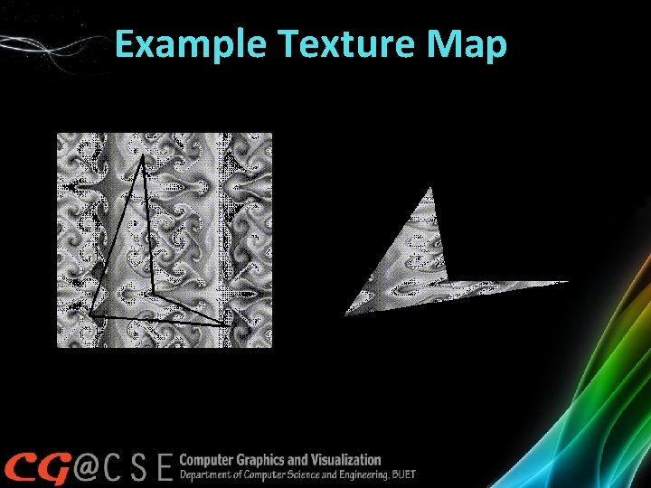
Example Texture Map

Types of Textures �Bitmap textures �Bitmapped representation of images �Represented by an array � Color 3 texture(float s, float t){ � Return txtr[(int)(s*c), (int)(t*r)] �} �Procedural textures �Defined by a mathematical function �In either case, we have a ‘texture function’ �texture(s, t)

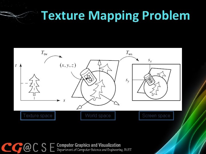
Texture Mapping Problem Texture space (sx, sy)=Tws(Ttw (s*, t*)) World space Screen space

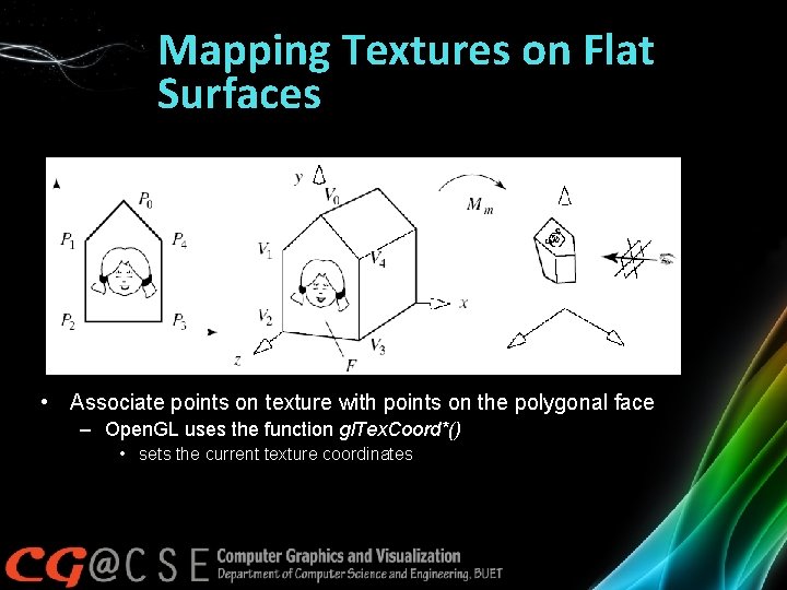
Mapping Textures on Flat Surfaces • Associate points on texture with points on the polygonal face – Open. GL uses the function gl. Tex. Coord*() • sets the current texture coordinates

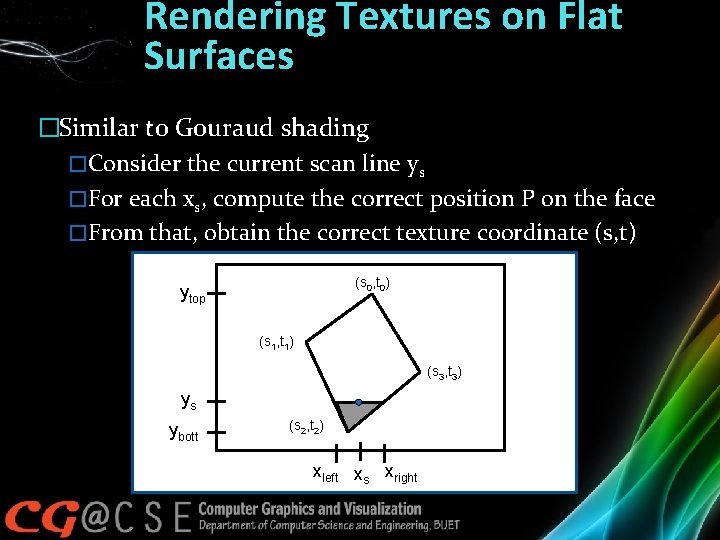
Rendering Textures on Flat Surfaces �Similar to Gouraud shading �Consider the current scan line ys �For each xs, compute the correct position P on the face �From that, obtain the correct texture coordinate (s, t) (s 0, t 0) ytop (s 1, t 1) (s 3, t 3) ys ybott (s 2, t 2) xleft xs xright

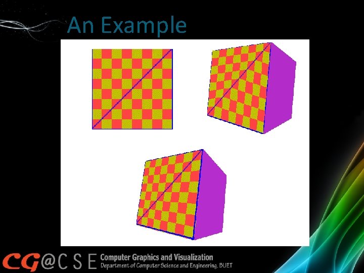
Caveat � Linear interpolation does not work always! � This is because… Equal steps across a projected space do not corresponds to equal steps across the 3 D space

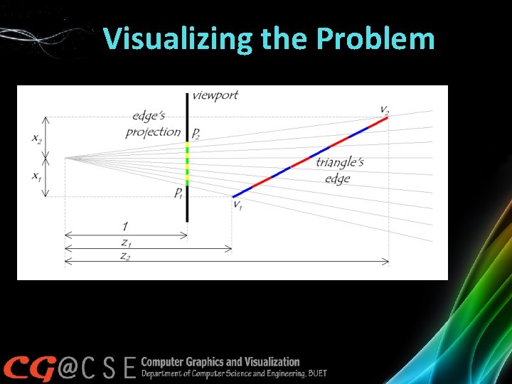
Visualizing the Problem Notice that uniform steps on the image plane do not correspond to uniform steps along the edge.

An Example

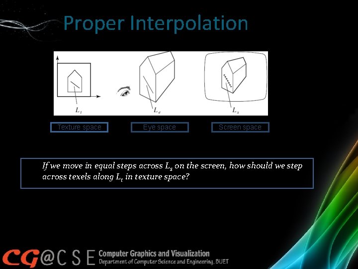
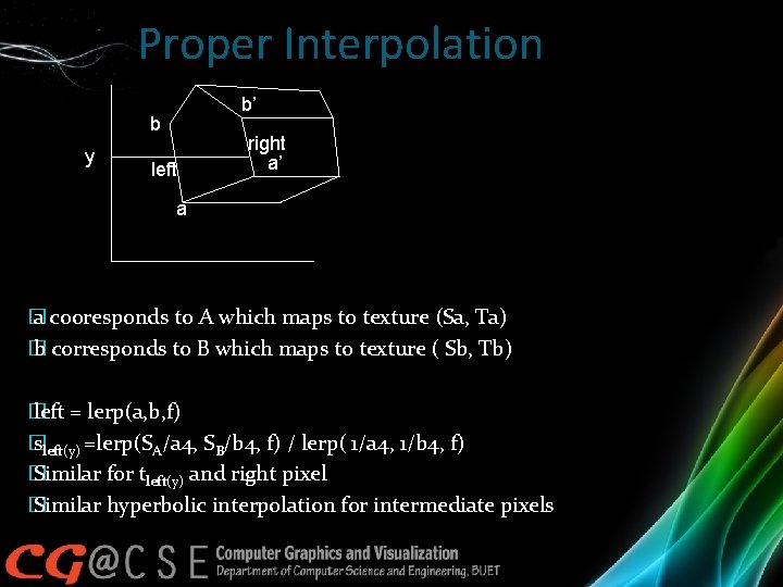
Proper Interpolation Texture space Eye space Screen space If we move in equal steps across Ls on the screen, how should we step across texels along Lt in texture space?

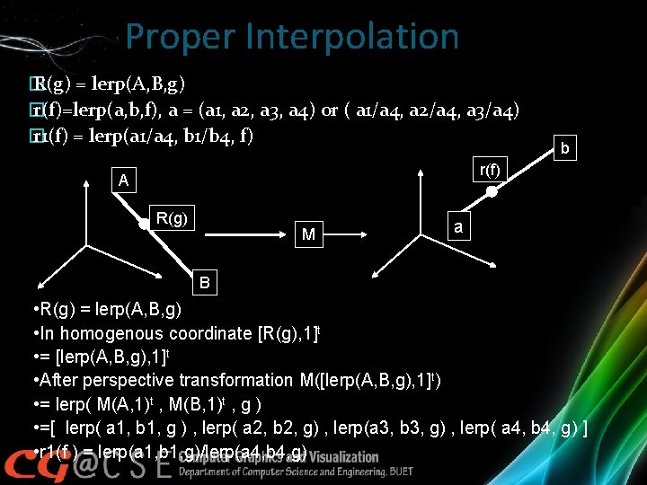
Proper Interpolation � R(g) = lerp(A, B, g) � r(f)=lerp(a, b, f), a = (a 1, a 2, a 3, a 4) or ( a 1/a 4, a 2/a 4, a 3/a 4) � r 1(f) = lerp(a 1/a 4, b 1/b 4, f) b r(f) A R(g) M a B • R(g) = lerp(A, B, g) • In homogenous coordinate [R(g), 1]t • = [lerp(A, B, g), 1]t • After perspective transformation M([lerp(A, B, g), 1]t) • = lerp( M(A, 1)t , M(B, 1)t , g ) • =[ lerp( a 1, b 1, g ) , lerp( a 2, b 2, g) , lerp(a 3, b 3, g) , lerp( a 4, b 4, g) ] • r 1(f ) = lerp(a 1, b 1, g)/lerp(a 4, b 4, g)

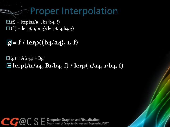
Proper Interpolation � r 1(f) = lerp(a 1/a 4, b 1/b 4, f) � r 1(f ) = lerp(a 1, b 1, g)/lerp(a 4, b 4, g) � g = f / lerp((b 4/a 4), 1, f) � R(g) = A(1 -g) + Bg � = lerp(A 1/a 4, B 1/b 4, f) / lerp( 1/a 4, 1/b 4, f)

Proper Interpolation b’ b y left right a’ a � a cooresponds to A which maps to texture (Sa, Ta) � b corresponds to B which maps to texture ( Sb, Tb) � left = lerp(a, b, f) � sleft(y) =lerp(SA/a 4, SB/b 4, f) / lerp( 1/a 4, 1/b 4, f) � Similar for tleft(y) and right pixel � Similar hyperbolic interpolation for intermediate pixels

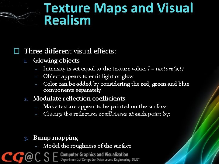
Texture Maps and Visual Realism � Three different visual effects: 1. Glowing objects – Intensity is set equal to the texture value: I = texture(s, t) – Object appears to emit light or glow – Color can be added by considering the red, green and blue components separately 2. Modulate reflection coefficients – Make texture appear to be painted on the surface – Change the reflection coefficients at each point by: 3. Bump mapping – Model the roughness of the surface

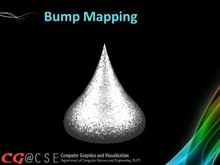
Bump Mapping

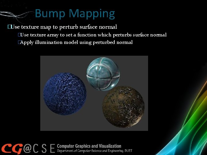
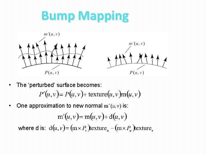
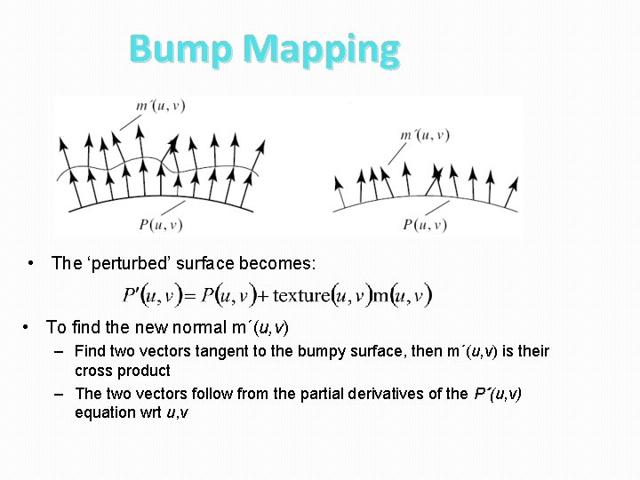
Bump Mapping �Use texture map to perturb surface normal �Use texture array to set a function which perturbs surface normal �Apply illumination model using perturbed normal

Bump Mapping • The ‘perturbed’ surface becomes: • One approximation to new normal m´(u, v) is: where d is:

Bump Mapping • The ‘perturbed’ surface becomes: • To find the new normal m´(u, v) – Find two vectors tangent to the bumpy surface, then m´(u, v) is their cross product – The two vectors follow from the partial derivatives of the P´(u, v) equation wrt u, v

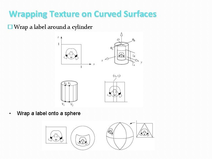
Wrapping Texture on Curved Surfaces � Wrap a label around a cylinder • Wrap a label onto a sphere

References �Hill 8. 5. 1 – 8. 5. 3, 8. 5. 5