CSE 373 NOVEMBER 13 TH MERGING AND PARTITIONING

CSE 373 NOVEMBER 13 TH – MERGING AND PARTITIONING
REVIEW • Slow sorts • O(n 2) • Insertion • Selection • Fast sorts • O(n log n) • Heap sort
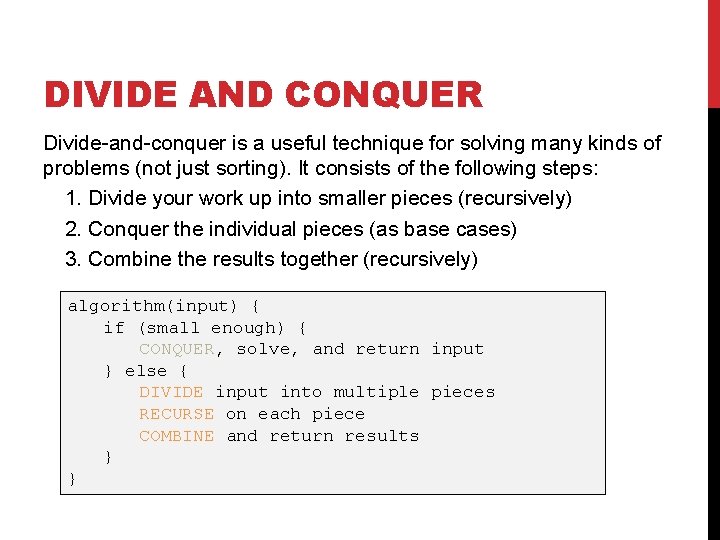
DIVIDE AND CONQUER Divide-and-conquer is a useful technique for solving many kinds of problems (not just sorting). It consists of the following steps: 1. Divide your work up into smaller pieces (recursively) 2. Conquer the individual pieces (as base cases) 3. Combine the results together (recursively) algorithm(input) { if (small enough) { CONQUER, solve, and return input } else { DIVIDE input into multiple pieces RECURSE on each piece COMBINE and return results } }
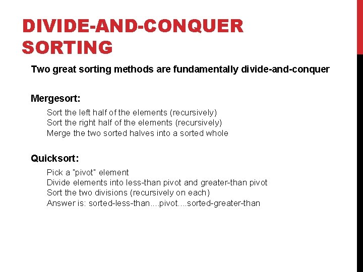
DIVIDE-AND-CONQUER SORTING Two great sorting methods are fundamentally divide-and-conquer Mergesort: Sort the left half of the elements (recursively) Sort the right half of the elements (recursively) Merge the two sorted halves into a sorted whole Quicksort: Pick a “pivot” element Divide elements into less-than pivot and greater-than pivot Sort the two divisions (recursively on each) Answer is: sorted-less-than. . pivot. . sorted-greater-than
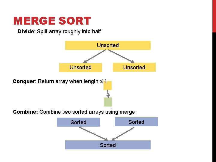
MERGE SORT Divide: Split array roughly into half Unsorted Conquer: Return array when length ≤ 1 Combine: Combine two sorted arrays using merge Sorted
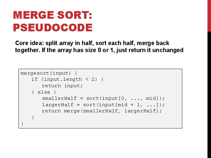
MERGE SORT: PSEUDOCODE Core idea: split array in half, sort each half, merge back together. If the array has size 0 or 1, just return it unchanged mergesort(input) { if (input. length < 2) { return input; } else { smaller. Half = sort(input[0, . . . , mid]); larger. Half = sort(input[mid + 1, . . . ]); return merge(smaller. Half, larger. Half); } }
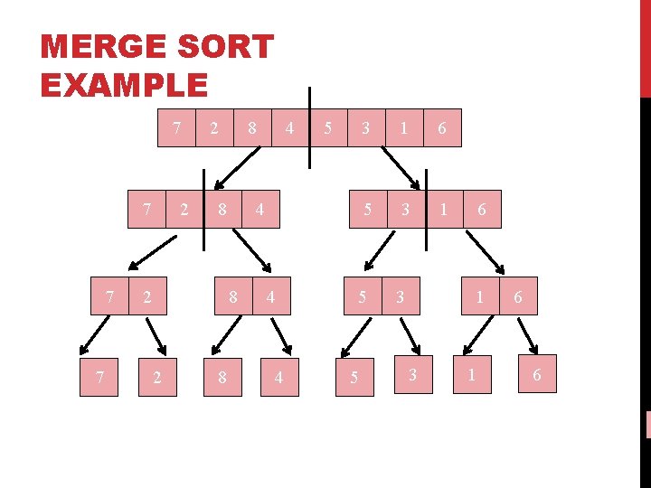
MERGE SORT EXAMPLE 7 7 2 2 8 8 2 8 5 4 8 2 4 4 4 3 1 6 5 3 1 5 5 3 6 1 3 1 6 6
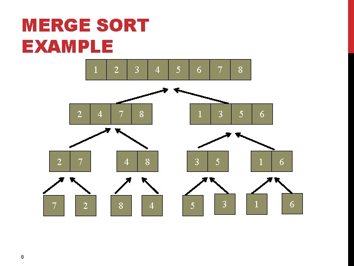
MERGE SORT EXAMPLE 1 2 2 7 8 4 2 3 7 7 8 5 8 4 2 4 8 4 6 7 8 1 3 5 5 6 1 3 1 6 6
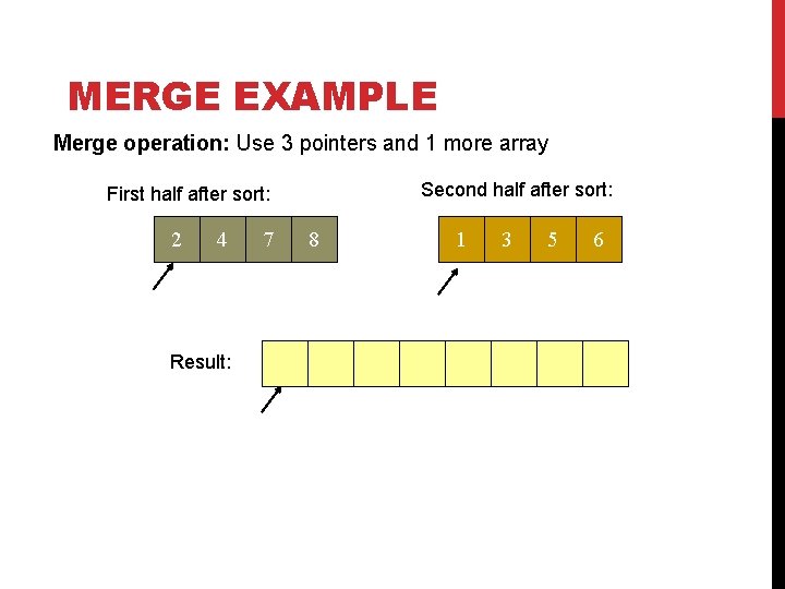
MERGE EXAMPLE Merge operation: Use 3 pointers and 1 more array Second half after sort: First half after sort: 2 4 Result: 7 8 1 3 5 6
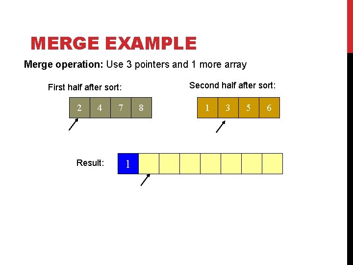
MERGE EXAMPLE Merge operation: Use 3 pointers and 1 more array Second half after sort: First half after sort: 2 4 Result: 7 8 1 1 3 5 6
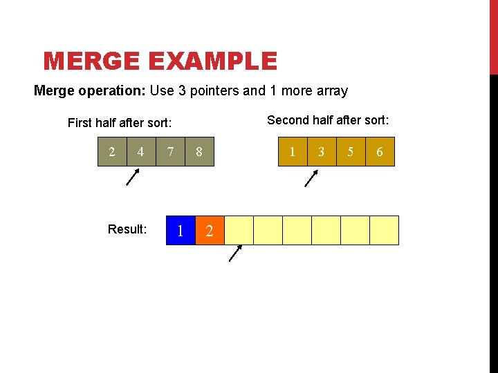
MERGE EXAMPLE Merge operation: Use 3 pointers and 1 more array Second half after sort: First half after sort: 2 4 Result: 7 8 1 1 2 3 5 6
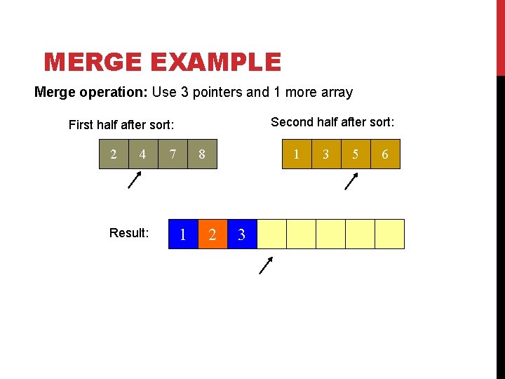
MERGE EXAMPLE Merge operation: Use 3 pointers and 1 more array Second half after sort: First half after sort: 2 4 Result: 7 8 1 1 2 3 3 5 6
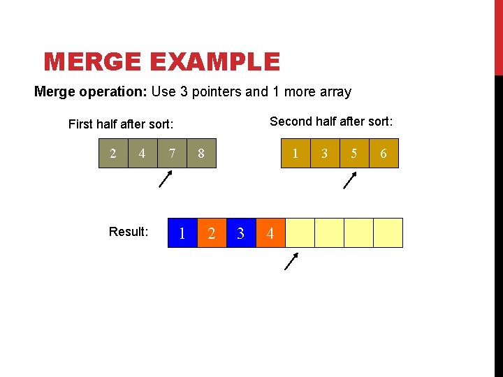
MERGE EXAMPLE Merge operation: Use 3 pointers and 1 more array Second half after sort: First half after sort: 2 4 Result: 7 8 1 1 2 3 4 3 5 6
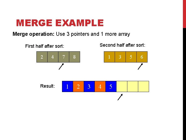
MERGE EXAMPLE Merge operation: Use 3 pointers and 1 more array Second half after sort: First half after sort: 2 4 Result: 7 8 1 1 2 3 4 5 3 5 6
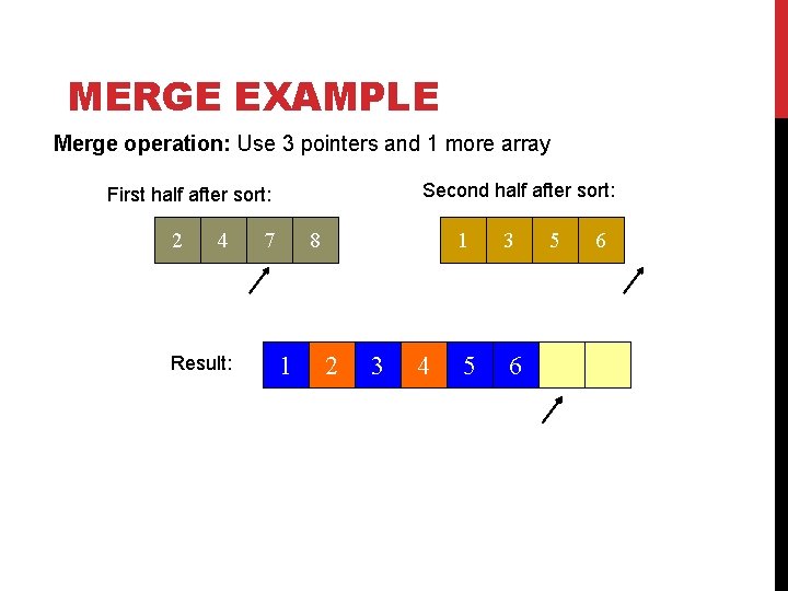
MERGE EXAMPLE Merge operation: Use 3 pointers and 1 more array Second half after sort: First half after sort: 2 4 Result: 7 8 1 2 3 4 1 3 5 6
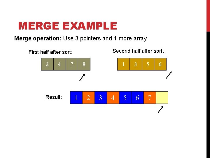
MERGE EXAMPLE Merge operation: Use 3 pointers and 1 more array Second half after sort: First half after sort: 2 4 Result: 7 8 1 2 3 4 1 3 5 5 6 7 6
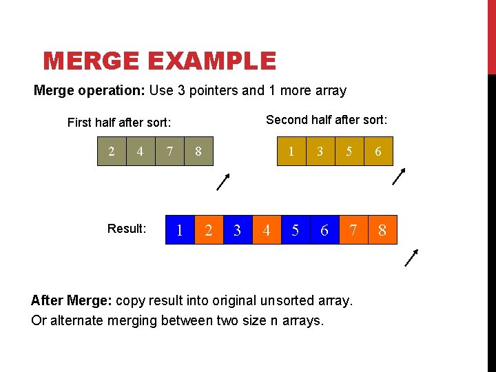
MERGE EXAMPLE Merge operation: Use 3 pointers and 1 more array Second half after sort: First half after sort: 2 4 Result: 7 8 1 2 3 4 1 3 5 6 7 8 After Merge: copy result into original unsorted array. Or alternate merging between two size n arrays.
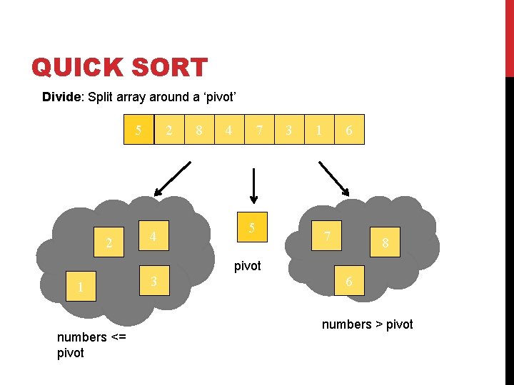
QUICK SORT Divide: Split array around a ‘pivot’ 5 2 2 4 8 4 7 5 3 1 6 7 8 pivot 1 numbers <= pivot 3 6 numbers > pivot
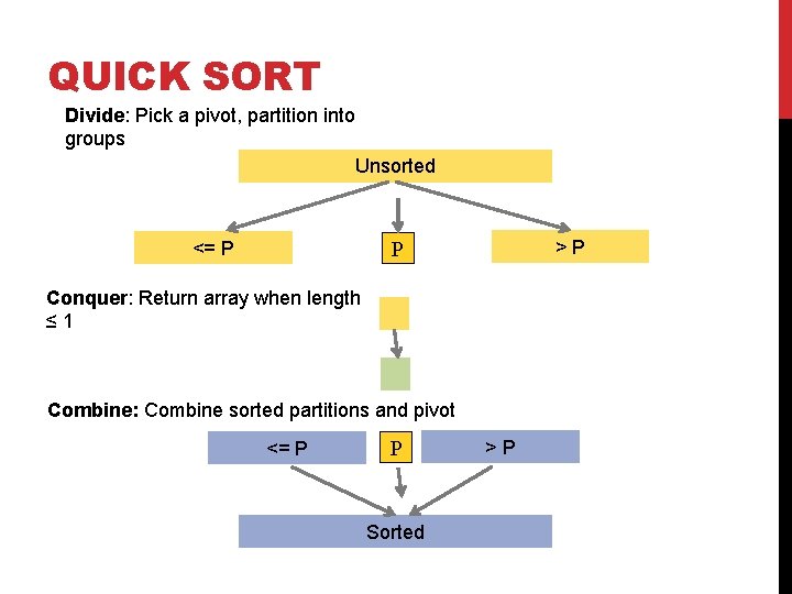
QUICK SORT Divide: Pick a pivot, partition into groups Unsorted >P P <= P Conquer: Return array when length ≤ 1 Combine: Combine sorted partitions and pivot <= P P Sorted >P
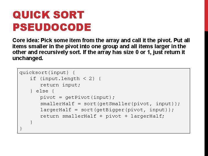
QUICK SORT PSEUDOCODE Core idea: Pick some item from the array and call it the pivot. Put all items smaller in the pivot into one group and all items larger in the other and recursively sort. If the array has size 0 or 1, just return it unchanged. quicksort(input) { if (input. length < 2) { return input; } else { pivot = get. Pivot(input); smaller. Half = sort(get. Smaller(pivot, input)); larger. Half = sort(get. Bigger(pivot, input)); return smaller. Half + pivot + larger. Half; } }
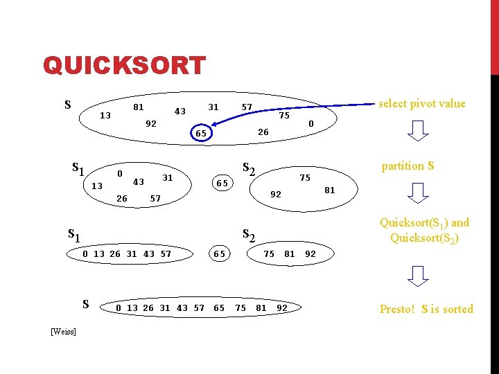
QUICKSORT S 81 13 S 1 92 0 13 26 31 43 65 S 2 select pivot value 0 S 65 0 13 26 31 43 57 65 81 Quicksort(S 1) and Quicksort(S 2) S 2 0 13 26 31 43 57 partition S 75 92 57 S 1 [Weiss] 75 26 65 31 43 57 75 81 92 Presto! S is sorted
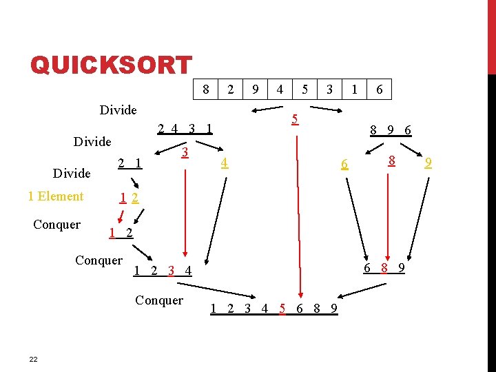
QUICKSORT 8 2 Divide 1 Element Conquer 2 1 3 5 1 3 4 6 8 9 6 6 8 12 1 2 Conquer 6 8 9 1 2 3 4 Conquer 22 4 5 2 4 3 1 Divide 9 1 2 3 4 5 6 8 9 9
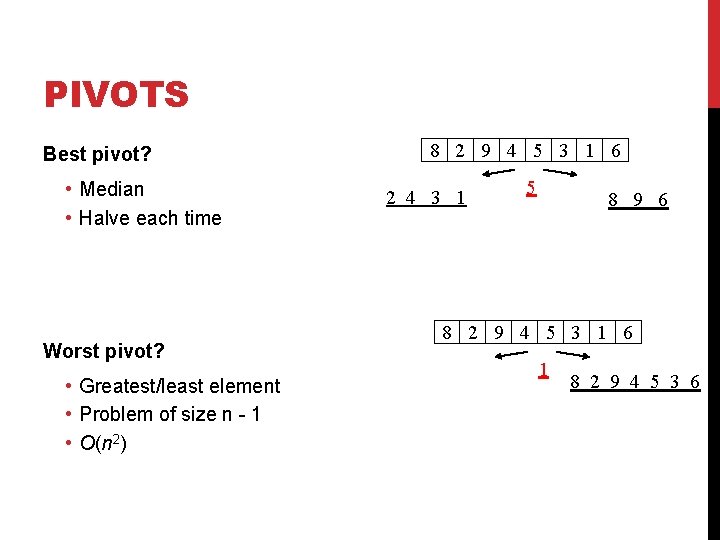
PIVOTS Best pivot? • Median • Halve each time Worst pivot? • Greatest/least element • Problem of size n - 1 • O(n 2) 8 2 9 4 5 3 1 6 2 4 3 1 5 8 9 6 8 2 9 4 5 3 1 6 1 8 2 9 4 5 3 6
![POTENTIAL PIVOT RULES While sorting arr from lo (inclusive) to hi (exclusive)… Pick arr[lo] POTENTIAL PIVOT RULES While sorting arr from lo (inclusive) to hi (exclusive)… Pick arr[lo]](http://slidetodoc.com/presentation_image_h2/8cf899f525fb374a2de3c79929ec7551/image-24.jpg)
POTENTIAL PIVOT RULES While sorting arr from lo (inclusive) to hi (exclusive)… Pick arr[lo] or arr[hi-1] • Fast, but worst-case occurs with mostly sorted input Pick random element in the range • Does as well as any technique, but (pseudo)random number generation can be slow • Still probably the most elegant approach Median of 3, e. g. , arr[lo], arr[hi-1], arr[(hi+lo)/2] • Common heuristic that tends to work well
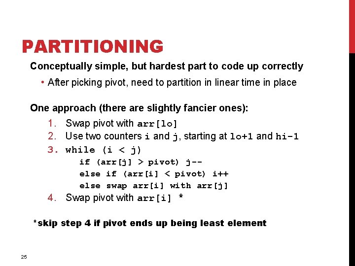
PARTITIONING Conceptually simple, but hardest part to code up correctly • After picking pivot, need to partition in linear time in place One approach (there are slightly fancier ones): 1. Swap pivot with arr[lo] 2. Use two counters i and j, starting at lo+1 and hi-1 3. while (i < j) if (arr[j] > pivot) j-else if (arr[i] < pivot) i++ else swap arr[i] with arr[j] 4. Swap pivot with arr[i] * *skip step 4 if pivot ends up being least element 25
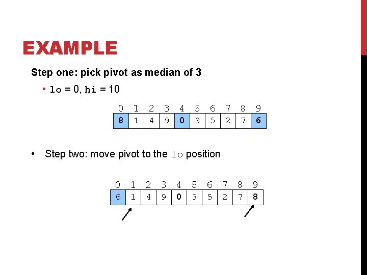
EXAMPLE Step one: pick pivot as median of 3 • lo = 0, hi = 10 0 1 2 3 4 5 6 7 8 9 8 1 4 9 0 3 5 2 7 6 • Step two: move pivot to the lo position 0 1 2 3 4 5 6 7 8 9 6 1 4 9 0 3 5 2 7 8
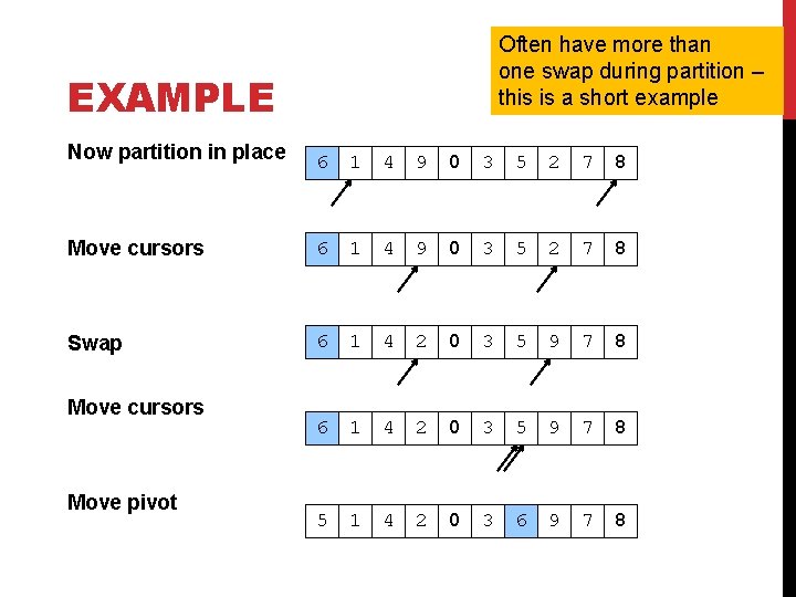
Often have more than one swap during partition – this is a short example EXAMPLE Now partition in place 6 1 4 9 0 3 5 2 7 8 Move cursors 6 1 4 9 0 3 5 2 7 8 Swap 6 1 4 2 0 3 5 9 7 8 5 1 4 2 0 3 6 9 7 8 Move cursors Move pivot
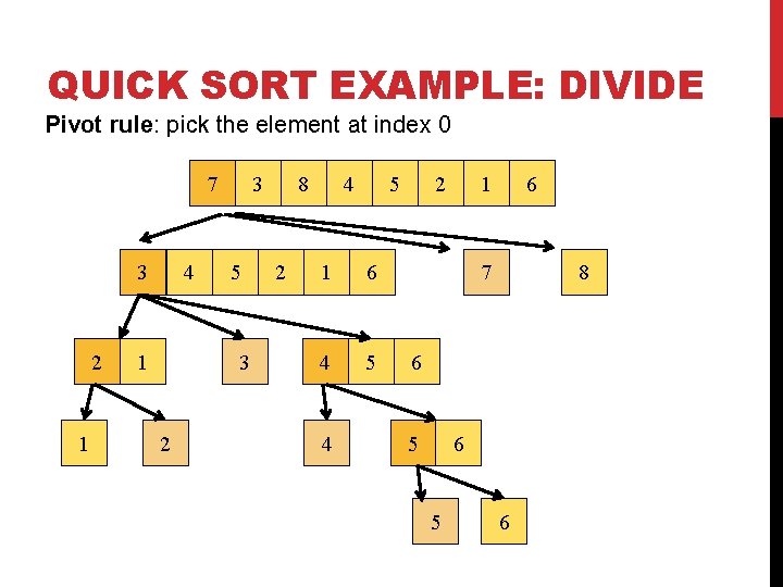
QUICK SORT EXAMPLE: DIVIDE Pivot rule: pick the element at index 0 7 3 2 1 4 1 3 5 3 2 8 2 4 5 1 6 4 5 4 2 1 6 7 8 6 5 6
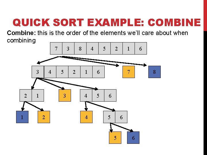
QUICK SORT EXAMPLE: COMBINE Combine: this is the order of the elements we’ll care about when combining 7 3 2 1 4 1 3 5 3 2 8 2 4 5 1 6 4 5 4 2 1 6 7 8 6 5 6
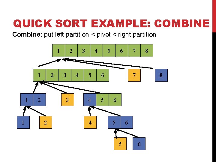
QUICK SORT EXAMPLE: COMBINE Combine: put left partition < pivot < right partition 1 1 2 2 2 3 3 2 3 4 4 5 5 6 4 5 4 6 7 8 6 5 6
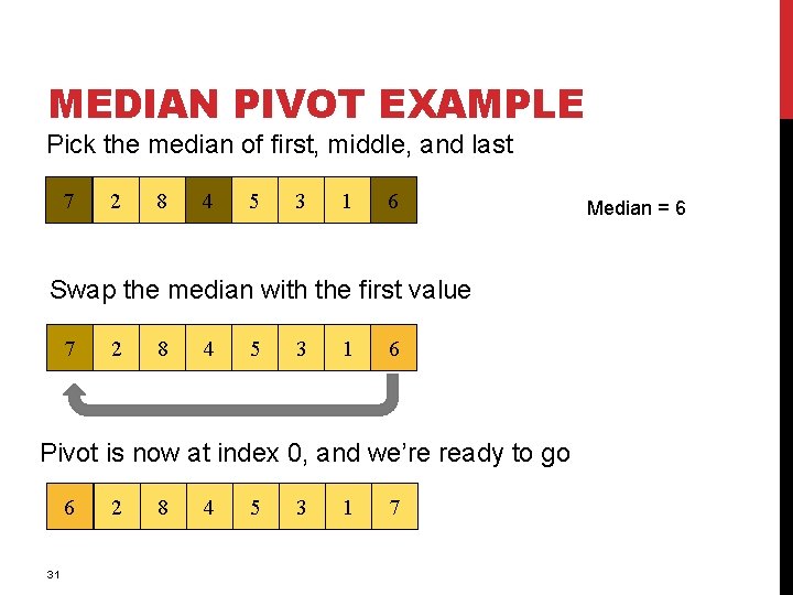
MEDIAN PIVOT EXAMPLE Pick the median of first, middle, and last 7 2 8 4 5 3 1 6 Swap the median with the first value 7 2 8 4 5 3 1 6 Pivot is now at index 0, and we’re ready to go 6 31 2 8 4 5 3 1 7 Median = 6
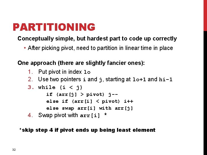
PARTITIONING Conceptually simple, but hardest part to code up correctly • After picking pivot, need to partition in linear time in place One approach (there are slightly fancier ones): 1. Put pivot in index lo 2. Use two pointers i and j, starting at lo+1 and hi-1 3. while (i < j) if (arr[j] > pivot) j-else if (arr[i] < pivot) i++ else swap arr[i] with arr[j] 4. Swap pivot with arr[i] * *skip step 4 if pivot ends up being least element 32
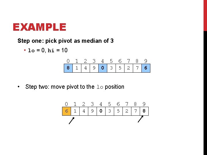
EXAMPLE Step one: pick pivot as median of 3 • lo = 0, hi = 10 0 1 2 3 4 5 6 7 8 9 8 1 4 9 0 3 5 2 7 6 • Step two: move pivot to the lo position 0 1 2 3 4 5 6 7 8 9 6 1 4 9 0 3 5 2 7 8
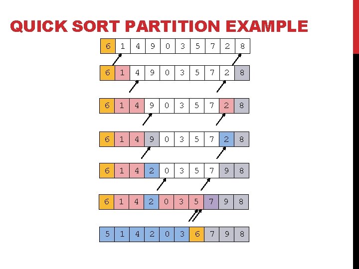
QUICK SORT PARTITION EXAMPLE 6 1 4 9 0 3 5 7 2 8 6 1 4 2 0 3 5 7 9 8 5 1 4 2 0 3 6 7 9 8
CUTOFFS For small n, all that recursion tends to cost more than doing a quadratic sort • Remember asymptotic complexity is for large n Common engineering technique: switch algorithm below a cutoff • Reasonable rule of thumb: use insertion sort for n < 10 Notes: • Could also use a cutoff for merge sort • Cutoffs are also the norm with parallel algorithms • Switch to sequential algorithm • None of this affects asymptotic complexity
QUICK SORT ANALYSIS Best-case: Pivot is always the median T(0)=T(1)=1 T(n)=2 T(n/2) + n -- linear-time partition Same recurrence as mergesort: O(n log n) Worst-case: Pivot is always smallest or largest element T(0)=T(1)=1 T(n) = 1 T(n-1) + n Basically same recurrence as selection sort: O(n 2) Average-case (e. g. , with random pivot) • O(n log n), not responsible for proof
HOW FAST CAN WE SORT? Heapsort & mergesort have O(n log n) worst-case running time Quicksort has O(n log n) average-case running time • Assuming our comparison model: The only operation an algorithm can perform on data items is a 2 -element comparison. There is no lower asymptotic complexity, such as O(n) or O(n log n)
COUNTING COMPARISONS No matter what the algorithm is, it cannot make progress without doing comparisons
COUNTING COMPARISONS No matter what the algorithm is, it cannot make progress without doing comparisons • Intuition: Each comparison can at best eliminate half the remaining possibilities of possible orderings
COUNTING COMPARISONS No matter what the algorithm is, it cannot make progress without doing comparisons • Intuition: Each comparison can at best eliminate half the remaining possibilities of possible orderings Can represent this process as a decision tree
COUNTING COMPARISONS No matter what the algorithm is, it cannot make progress without doing comparisons • Intuition: Each comparison can at best eliminate half the remaining possibilities of possible orderings Can represent this process as a decision tree • Nodes contain “set of remaining possibilities” • Edges are “answers from a comparison” • The algorithm does not actually build the tree; it’s what our proof uses to represent “the most the algorithm could know so far” as the algorithm progresses
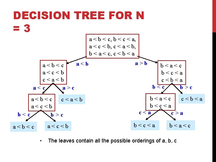
DECISION TREE FOR N =3 a < b < c, b < c < a, a < c < b, c < a < b, b < a < c, c < b < a a<b<c a<c<b c<a<b a<c a>c a<b<c c<a<b a<c<b b<c b>c a<c<b a<b<c • a>b b<a<c b<c<a c<b<a b<c b>c b<a<c c<b<a b<c<a c>a b<c<a b<a<c The leaves contain all the possible orderings of a, b, c
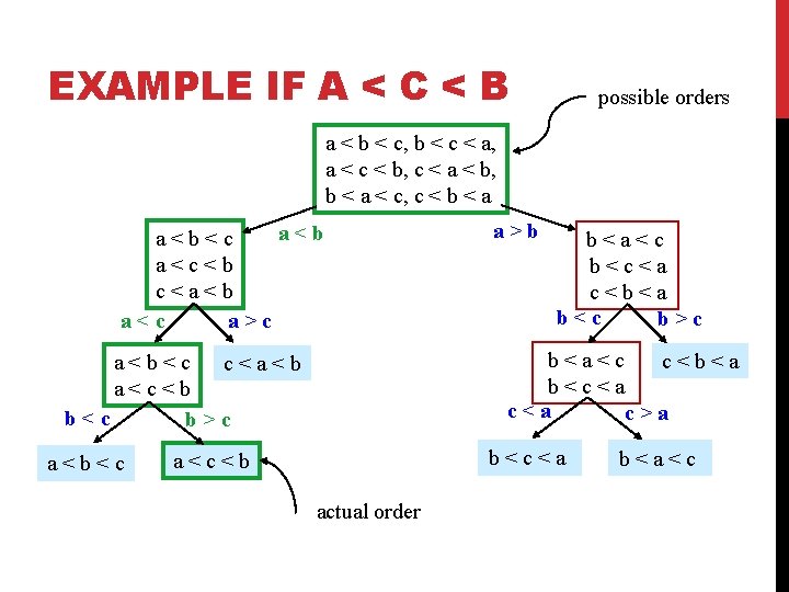
EXAMPLE IF A < C < B possible orders a < b < c, b < c < a, a < c < b, c < a < b, b < a < c, c < b < a a<b<c a<c<b c<a<b a<c a>c b<a<c b<c<a c<b<a b<c b>c b<a<c c<b<a b<c<a c>a a<b<c c<a<b a<c<b b<c b>c a<b<c a>b b<c<a a<c<b actual order b<a<c
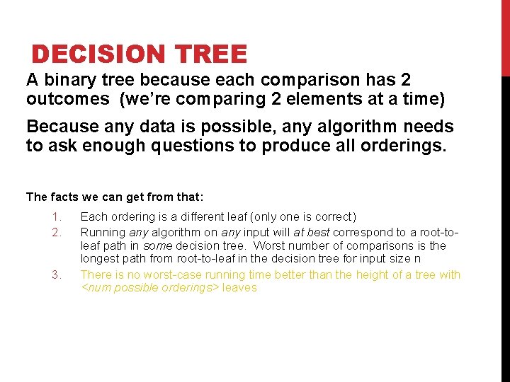
DECISION TREE A binary tree because each comparison has 2 outcomes (we’re comparing 2 elements at a time) Because any data is possible, any algorithm needs to ask enough questions to produce all orderings. The facts we can get from that: 1. 2. 3. Each ordering is a different leaf (only one is correct) Running any algorithm on any input will at best correspond to a root-toleaf path in some decision tree. Worst number of comparisons is the longest path from root-to-leaf in the decision tree for input size n There is no worst-case running time better than the height of a tree with <num possible orderings> leaves
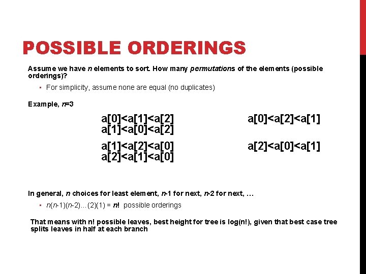
POSSIBLE ORDERINGS Assume we have n elements to sort. How many permutations of the elements (possible orderings)? • For simplicity, assume none are equal (no duplicates) Example, n=3 a[0]<a[1]<a[2] a[1]<a[0]<a[2] a[1]<a[2]<a[0] a[2]<a[1]<a[0]<a[2]<a[1] a[2]<a[0]<a[1] In general, n choices for least element, n-1 for next, n-2 for next, … • n(n-1)(n-2)…(2)(1) = n! possible orderings That means with n! possible leaves, best height for tree is log(n!), given that best case tree splits leaves in half at each branch
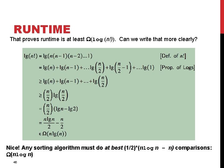
RUNTIME That proves runtime is at least (log (n!)). Can we write that more clearly? Nice! Any sorting algorithm must do at best (1/2)*(nlog n – n) comparisons: (nlog n) 46
SORTING • This is the lower bound for comparison sorts
SORTING • This is the lower bound for comparison sorts • How can non-comparison sorts work better?
SORTING • This is the lower bound for comparison sorts • How can non-comparison sorts work better? • They need to know something about the data
SORTING • This is the lower bound for comparison sorts • How can non-comparison sorts work better? • They need to know something about the data • Strings and Ints are very well ordered
- Slides: 50