CSE 373 Data Structures and Algorithms Lecture 17

CSE 373: Data Structures and Algorithms Lecture 17: Hashing II 1

Hash versus tree • Which is better, a hash set or a tree set? Hash Tree 2

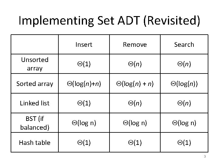
Implementing Set ADT (Revisited) Insert Remove Search Unsorted array (1) (n) Sorted array (log(n)+n) (log(n) + n) (log(n)) Linked list (1) (n) BST (if balanced) (log n) Hash table (1) 3

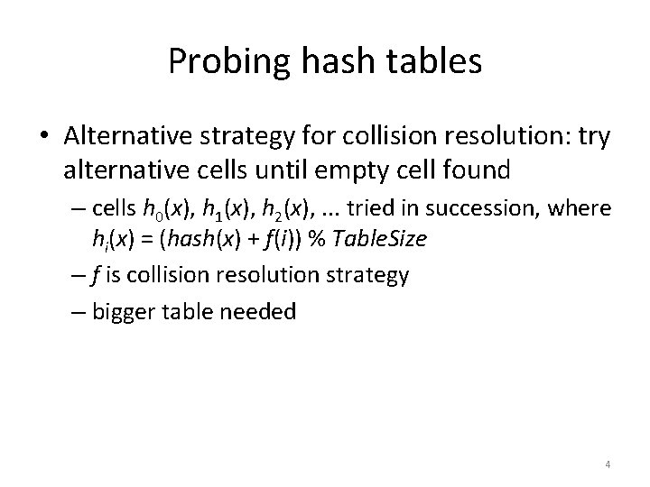
Probing hash tables • Alternative strategy for collision resolution: try alternative cells until empty cell found – cells h 0(x), h 1(x), h 2(x), . . . tried in succession, where hi(x) = (hash(x) + f(i)) % Table. Size – f is collision resolution strategy – bigger table needed 4

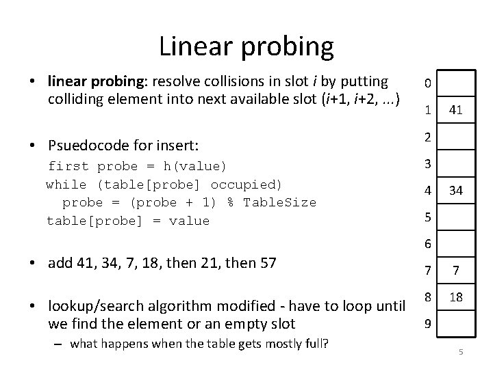
Linear probing • linear probing: resolve collisions in slot i by putting colliding element into next available slot (i+1, i+2, . . . ) • Psuedocode for insert: first probe = h(value) while (table[probe] occupied) probe = (probe + 1) % Table. Size table[probe] = value 0 1 41 2 3 4 34 5 6 • add 41, 34, 7, 18, then 21, then 57 • lookup/search algorithm modified - have to loop until we find the element or an empty slot – what happens when the table gets mostly full? 7 7 8 18 9 5

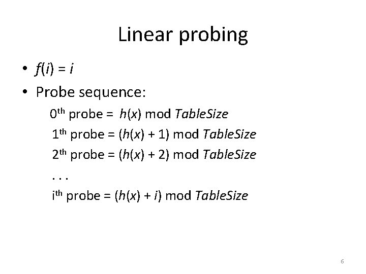
Linear probing • f(i) = i • Probe sequence: 0 th probe = h(x) mod Table. Size 1 th probe = (h(x) + 1) mod Table. Size 2 th probe = (h(x) + 2) mod Table. Size. . . ith probe = (h(x) + i) mod Table. Size 6

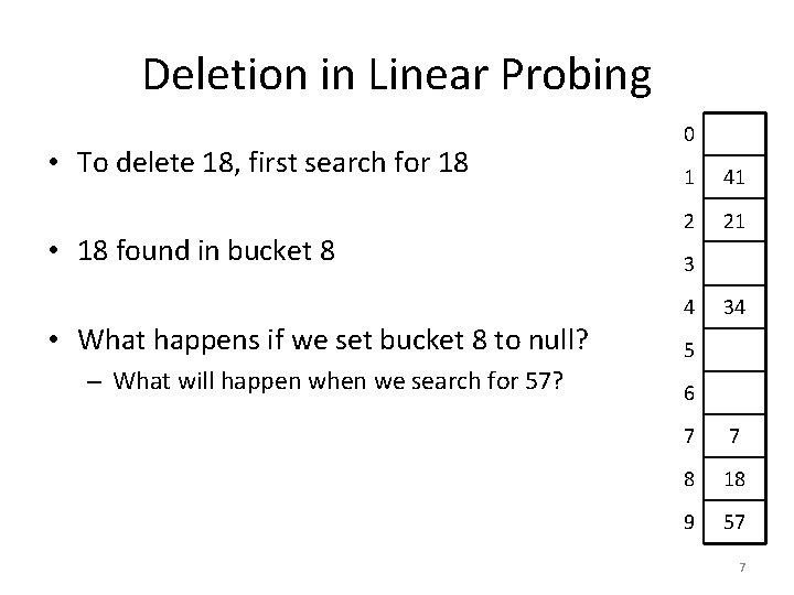
Deletion in Linear Probing • To delete 18, first search for 18 • 18 found in bucket 8 0 1 41 2 21 3 4 • What happens if we set bucket 8 to null? – What will happen when we search for 57? 34 5 6 7 7 8 18 9 57 7

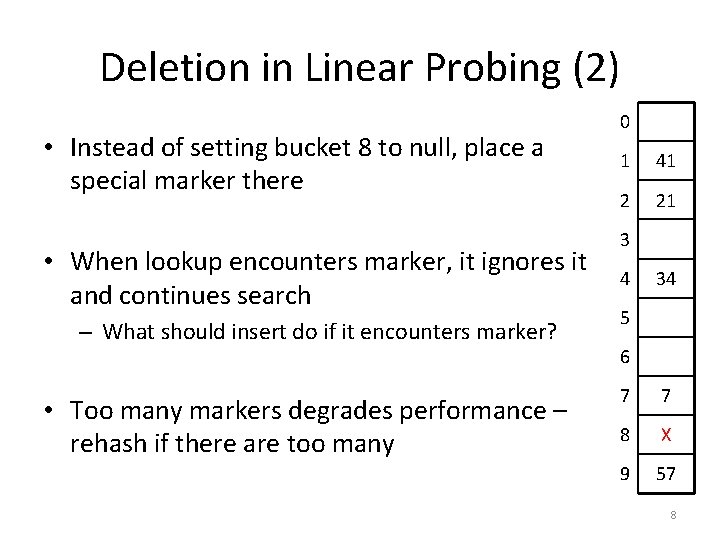
Deletion in Linear Probing (2) • Instead of setting bucket 8 to null, place a special marker there • When lookup encounters marker, it ignores it and continues search – What should insert do if it encounters marker? • Too many markers degrades performance – rehash if there are too many 0 1 41 2 21 3 4 34 5 6 7 7 8 X 9 57 8

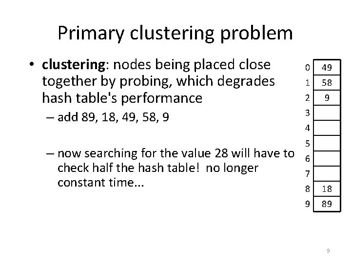
Primary clustering problem • clustering: nodes being placed close together by probing, which degrades hash table's performance – add 89, 18, 49, 58, 9 – now searching for the value 28 will have to check half the hash table! no longer constant time. . . 0 49 1 58 2 9 3 4 5 6 7 8 18 9 89 9

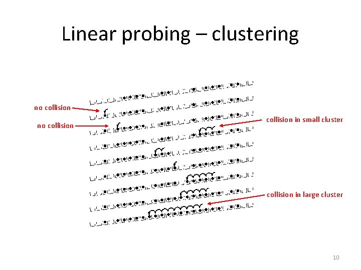
Linear probing – clustering no collision in small cluster collision in large cluster 10

Alternative probing strategy • Primary clustering occurs with linear probing because the same linear pattern: – if a slot is inside a cluster, then the next slot must either: • also be in that cluster, or • expand the cluster • Instead of searching forward in a linear fashion, consider searching forward using a quadratic function 11

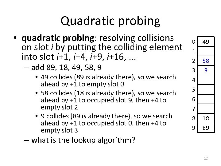
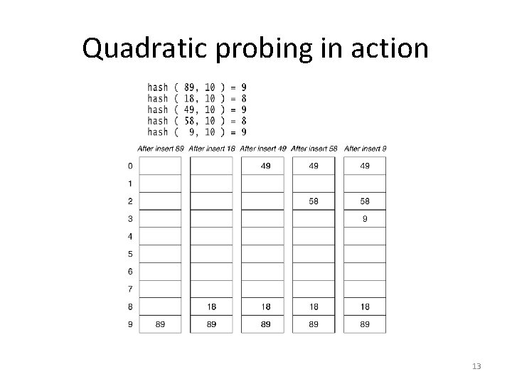
Quadratic probing • quadratic probing: resolving collisions on slot i by putting the colliding element into slot i+1, i+4, i+9, i+16, . . . – add 89, 18, 49, 58, 9 • 49 collides (89 is already there), so we search ahead by +1 to empty slot 0 • 58 collides (18 is already there), so we search ahead by +1 to occupied slot 9, then +4 to empty slot 2 • 9 collides (89 is already there), so we search ahead by +1 to occupied slot 0, then +4 to empty slot 3 0 49 1 2 58 3 9 4 5 6 7 8 18 9 89 – what is the lookup algorithm? 12

Quadratic probing in action 13

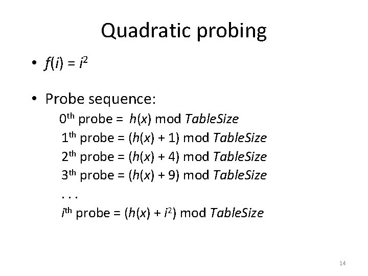
Quadratic probing • f(i) = i 2 • Probe sequence: 0 th probe = h(x) mod Table. Size 1 th probe = (h(x) + 1) mod Table. Size 2 th probe = (h(x) + 4) mod Table. Size 3 th probe = (h(x) + 9) mod Table. Size. . . ith probe = (h(x) + i 2) mod Table. Size 14

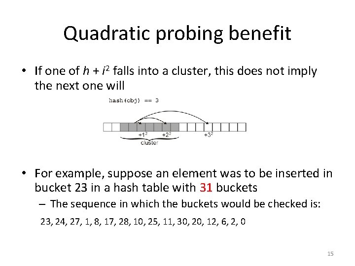
Quadratic probing benefit • If one of h + i 2 falls into a cluster, this does not imply the next one will • For example, suppose an element was to be inserted in bucket 23 in a hash table with 31 buckets – The sequence in which the buckets would be checked is: 23, 24, 27, 1, 8, 17, 28, 10, 25, 11, 30, 20, 12, 6, 2, 0 15

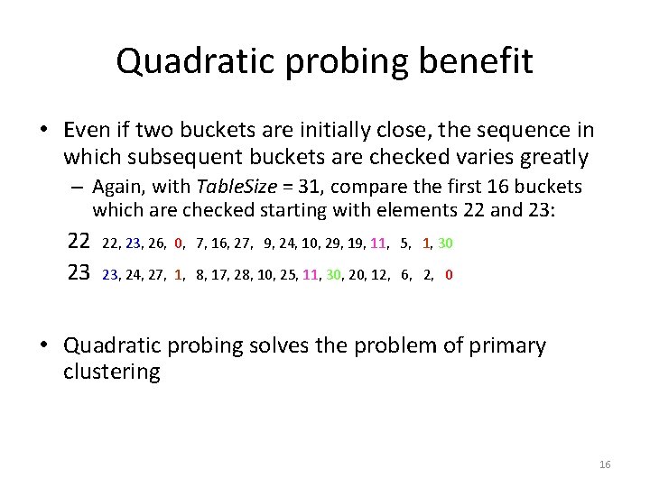
Quadratic probing benefit • Even if two buckets are initially close, the sequence in which subsequent buckets are checked varies greatly – Again, with Table. Size = 31, compare the first 16 buckets which are checked starting with elements 22 and 23: 22 23 22, 23, 26, 0, 7, 16, 27, 9, 24, 10, 29, 11, 5, 1, 30 23, 24, 27, 1, 8, 17, 28, 10, 25, 11, 30, 20, 12, 6, 2, 0 • Quadratic probing solves the problem of primary clustering 16

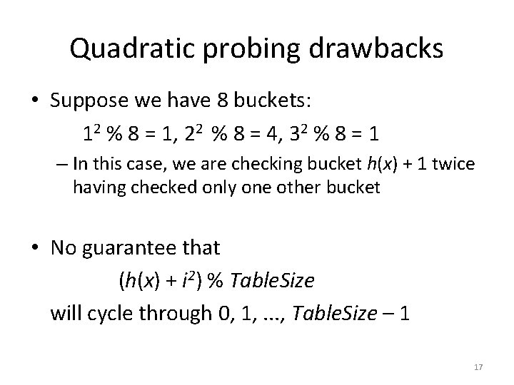
Quadratic probing drawbacks • Suppose we have 8 buckets: 12 % 8 = 1, 22 % 8 = 4, 32 % 8 = 1 – In this case, we are checking bucket h(x) + 1 twice having checked only one other bucket • No guarantee that (h(x) + i 2) % Table. Size will cycle through 0, 1, . . . , Table. Size – 1 17

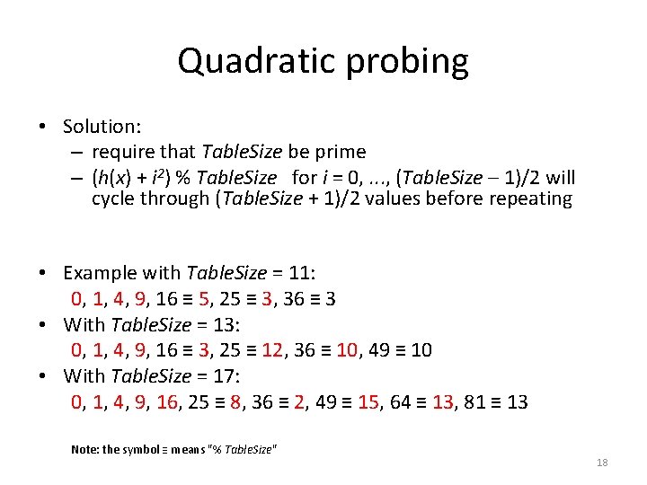
Quadratic probing • Solution: – require that Table. Size be prime – (h(x) + i 2) % Table. Size for i = 0, . . . , (Table. Size – 1)/2 will cycle through (Table. Size + 1)/2 values before repeating • Example with Table. Size = 11: 0, 1, 4, 9, 16 ≡ 5, 25 ≡ 3, 36 ≡ 3 • With Table. Size = 13: 0, 1, 4, 9, 16 ≡ 3, 25 ≡ 12, 36 ≡ 10, 49 ≡ 10 • With Table. Size = 17: 0, 1, 4, 9, 16, 25 ≡ 8, 36 ≡ 2, 49 ≡ 15, 64 ≡ 13, 81 ≡ 13 Note: the symbol ≡ means "% Table. Size" 18

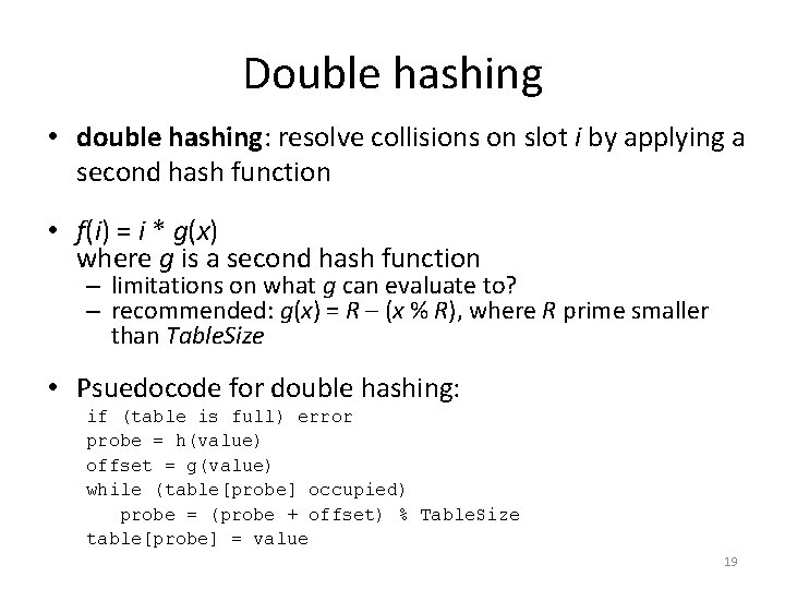
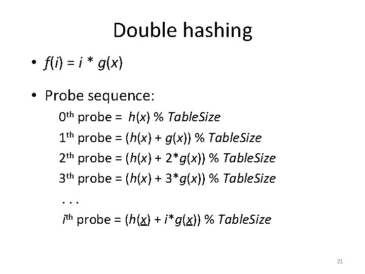
Double hashing • double hashing: resolve collisions on slot i by applying a second hash function • f(i) = i * g(x) where g is a second hash function – limitations on what g can evaluate to? – recommended: g(x) = R – (x % R), where R prime smaller than Table. Size • Psuedocode for double hashing: if (table is full) error probe = h(value) offset = g(value) while (table[probe] occupied) probe = (probe + offset) % Table. Size table[probe] = value 19

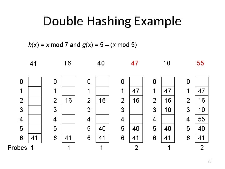
Double Hashing Example h(x) = x mod 7 and g(x) = 5 – (x mod 5) 16 41 0 1 2 3 4 5 6 41 Probes 1 0 1 2 3 4 5 6 16 41 1 40 0 1 2 3 4 5 6 16 40 41 1 47 0 1 2 3 4 5 6 47 16 40 41 2 10 0 1 2 3 4 5 6 47 16 10 40 41 1 55 0 1 2 3 4 5 6 47 16 10 55 40 41 2 20

Double hashing • f(i) = i * g(x) • Probe sequence: 0 th probe = h(x) % Table. Size 1 th probe = (h(x) + g(x)) % Table. Size 2 th probe = (h(x) + 2*g(x)) % Table. Size 3 th probe = (h(x) + 3*g(x)) % Table. Size. . . ith probe = (h(x) + i*g(x)) % Table. Size 21

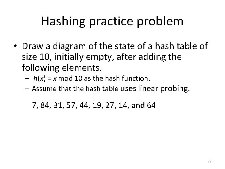
Hashing practice problem • Draw a diagram of the state of a hash table of size 10, initially empty, after adding the following elements. – h(x) = x mod 10 as the hash function. – Assume that the hash table uses linear probing. 7, 84, 31, 57, 44, 19, 27, 14, and 64 22

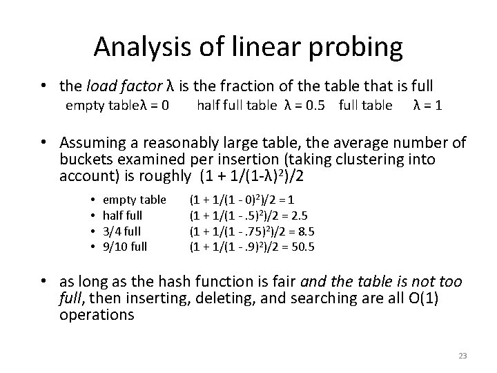
Analysis of linear probing • the load factor λ is the fraction of the table that is full empty tableλ = 0 half full table λ = 0. 5 full table λ=1 • Assuming a reasonably large table, the average number of buckets examined per insertion (taking clustering into account) is roughly (1 + 1/(1 -λ)2)/2 • • empty table half full 3/4 full 9/10 full (1 + 1/(1 - 0)2)/2 = 1 (1 + 1/(1 -. 5)2)/2 = 2. 5 (1 + 1/(1 -. 75)2)/2 = 8. 5 (1 + 1/(1 -. 9)2)/2 = 50. 5 • as long as the hash function is fair and the table is not too full, then inserting, deleting, and searching are all O(1) operations 23

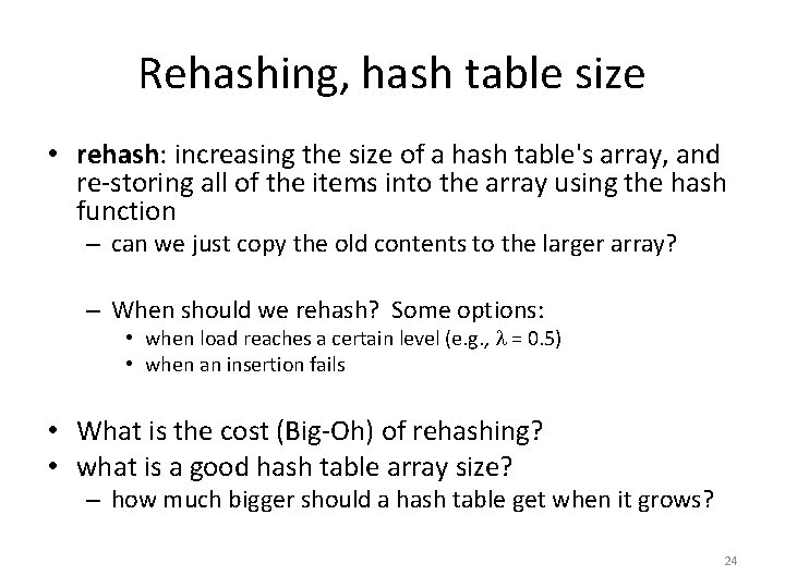
Rehashing, hash table size • rehash: increasing the size of a hash table's array, and re-storing all of the items into the array using the hash function – can we just copy the old contents to the larger array? – When should we rehash? Some options: • when load reaches a certain level (e. g. , = 0. 5) • when an insertion fails • What is the cost (Big-Oh) of rehashing? • what is a good hash table array size? – how much bigger should a hash table get when it grows? 24

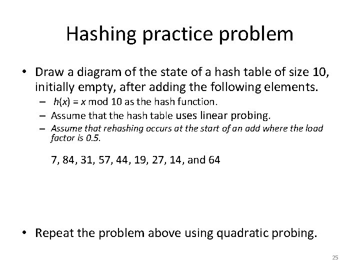
Hashing practice problem • Draw a diagram of the state of a hash table of size 10, initially empty, after adding the following elements. – h(x) = x mod 10 as the hash function. – Assume that the hash table uses linear probing. – Assume that rehashing occurs at the start of an add where the load factor is 0. 5. 7, 84, 31, 57, 44, 19, 27, 14, and 64 • Repeat the problem above using quadratic probing. 25