CSE 332 Parallel Sorting Richard Anderson Spring 2016

CSE 332: Parallel Sorting Richard Anderson Spring 2016 1

Announcements 2

Recap Last lectures – simple parallel programs – common patterns: map, reduce – analysis tools (work, span, parallelism) Now – Amdahl’s Law – Parallel quicksort, merge sort – useful building blocks: prefix, pack 3

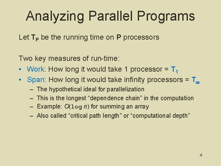
Analyzing Parallel Programs Let TP be the running time on P processors Two key measures of run-time: • Work: How long it would take 1 processor = T 1 • Span: How long it would take infinity processors = T – – The hypothetical ideal for parallelization This is the longest “dependence chain” in the computation Example: O(log n) for summing an array Also called “critical path length” or “computational depth” 4

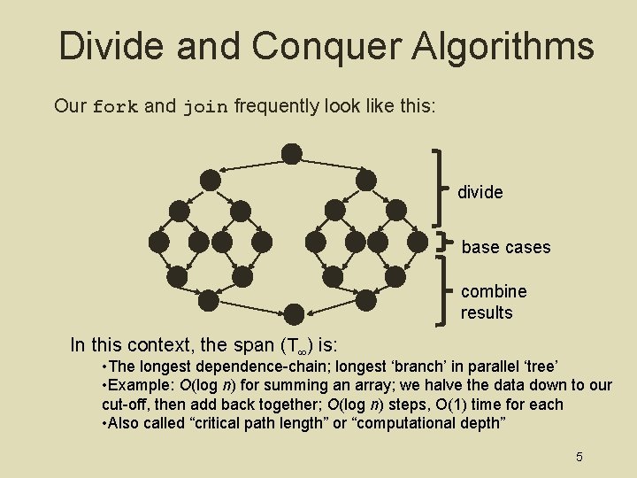
Divide and Conquer Algorithms Our fork and join frequently look like this: divide base cases combine results In this context, the span (T ) is: • The longest dependence-chain; longest ‘branch’ in parallel ‘tree’ • Example: O(log n) for summing an array; we halve the data down to our cut-off, then add back together; O(log n) steps, O(1) time for each • Also called “critical path length” or “computational depth” 5

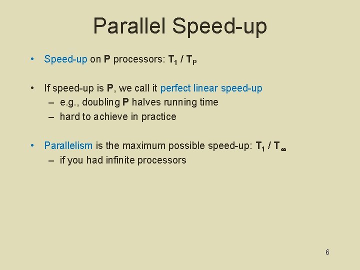
Parallel Speed-up • Speed-up on P processors: T 1 / TP • If speed-up is P, we call it perfect linear speed-up – e. g. , doubling P halves running time – hard to achieve in practice • Parallelism is the maximum possible speed-up: T 1 / T – if you had infinite processors 6

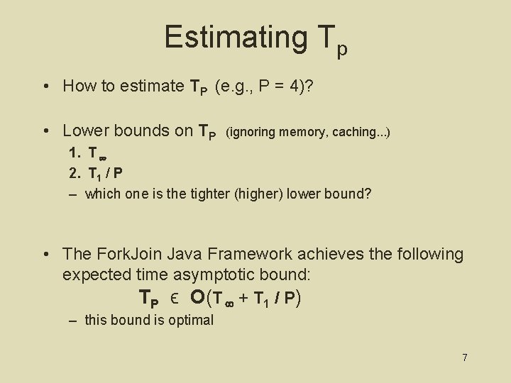
Estimating Tp • How to estimate TP (e. g. , P = 4)? • Lower bounds on TP (ignoring memory, caching. . . ) 1. T 2. T 1 / P – which one is the tighter (higher) lower bound? • The Fork. Join Java Framework achieves the following expected time asymptotic bound: TP ϵ O(T + T 1 / P) – this bound is optimal 7

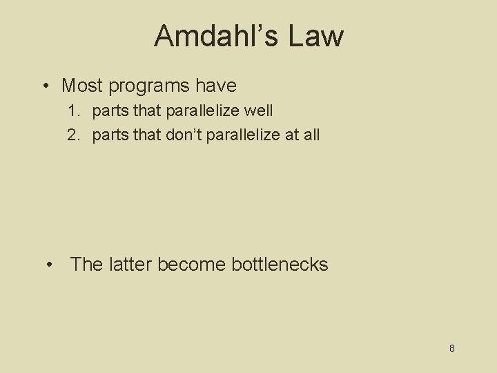
Amdahl’s Law • Most programs have 1. parts that parallelize well 2. parts that don’t parallelize at all • The latter become bottlenecks 8

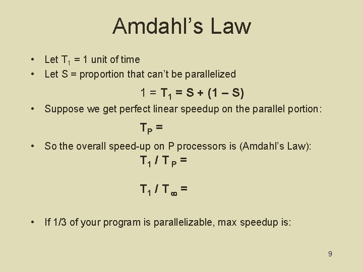
Amdahl’s Law • Let T 1 = 1 unit of time • Let S = proportion that can’t be parallelized 1 = T 1 = S + (1 – S) • Suppose we get perfect linear speedup on the parallel portion: TP = • So the overall speed-up on P processors is (Amdahl’s Law): T 1 / T P = T 1 / T = • If 1/3 of your program is parallelizable, max speedup is: 9

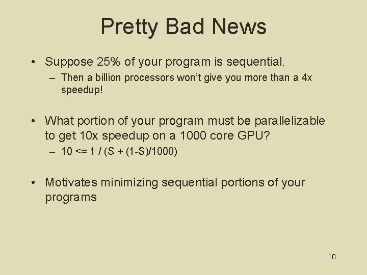
Pretty Bad News • Suppose 25% of your program is sequential. – Then a billion processors won’t give you more than a 4 x speedup! • What portion of your program must be parallelizable to get 10 x speedup on a 1000 core GPU? – 10 <= 1 / (S + (1 -S)/1000) • Motivates minimizing sequential portions of your programs 10

Take Aways • Parallel algorithms can be a big win • Many fit standard patterns that are easy to implement • Can’t just rely on more processors to make things faster (Amdahl’s Law) 11

Parallelizable? Fibonacci (N) 12

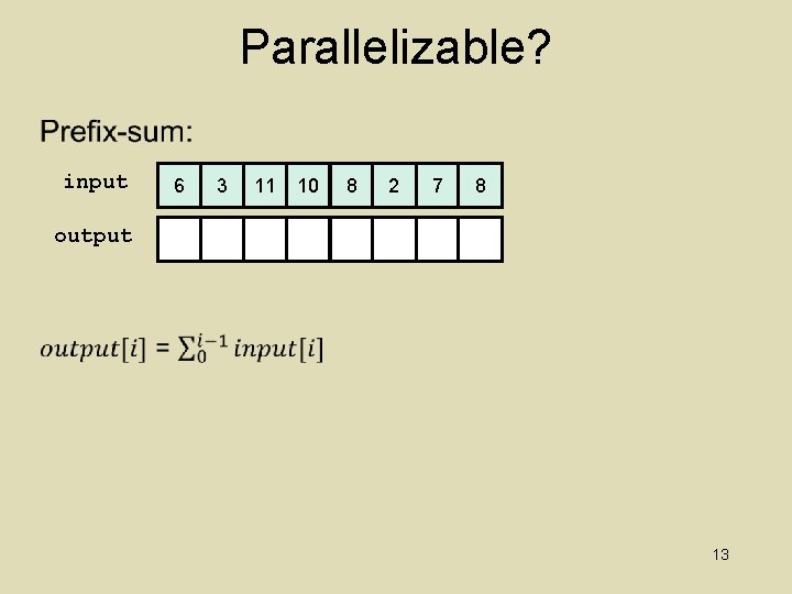
Parallelizable? input 6 3 11 10 8 2 7 8 output 13

First Pass: Sum [0, 7]: 6 3 11 10 8 2 7 8 14

First Pass: Sum [0, 7]: Sum [0, 3]: Sum [2, 3]: Sum [0, 1]: 6 Sum [4, 7]: 3 11 Sum [4, 5]: 10 8 Sum [5, 7]: 2 7 8 15

2 nd Pass: Use Sum for Prefix-Sum [0, 7]: Sum<0: Sum [0, 3]: Sum<0: Sum [2, 3]: Sum<2: Sum [0, 1]: Sum<0: 6 Sum [4, 7]: Sum<4: 3 11 Sum [4, 5]: Sum<4: 10 8 Sum [6, 7]: Sum<6: 2 7 8 16

2 nd Pass: Use Sum for Prefix-Sum [0, 7]: Sum<0: Sum [0, 3]: Sum<0: Sum [2, 3]: Sum<2: Sum [0, 1]: Sum<0: 6 3 11 10 Sum [4, 7]: Sum<4: Sum [4, 5]: Sum<4: 8 2 Sum [6, 7]: Sum<6: 7 8 Go from root down to leaves Root – sum<0 = Left-child – sum<K = Right-child – sum<K = 17

Prefix-Sum Analysis • First Pass (Sum): – span = • Second Pass: – single pass from root down to leaves • update children’s sum<K value based on parent and sibling – span = • Total – span = 18

Parallel Prefix, Generalized Prefix-sum is another common pattern (prefix problems) – – maximum element to the left of i is there an element to the left of i i satisfying some property? count of elements to the left of i satisfying some property … We can solve all of these problems in the same way 19

Pack: input 6 3 11 10 8 2 7 8 test: X < 8? output Output array of elements satisfying test, in original order 20

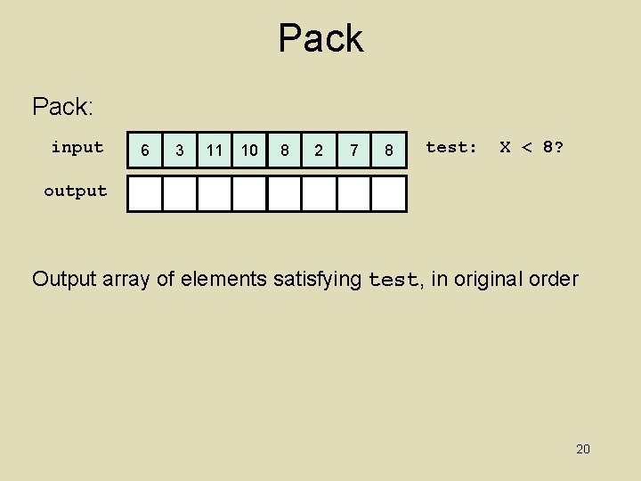
Parallel Pack? Pack input 6 3 11 10 output 6 3 2 7 8 test: X < 8? • Determining which elements to include is easy • Determining where each element goes in output is hard – seems to depend on previous results 21

Parallel Pack 1. map test input, output [0, 1] bit vector input 6 3 11 10 8 2 7 8 test 1 1 0 0 0 1 1 0 test: X < 8? 22

Parallel Pack 1. map test input, output [0, 1] bit vector input 6 3 11 10 8 2 7 8 test 1 1 0 0 0 1 1 0 test: X < 8? 2. transform bit vector into array of indices into result array pos 1 2 3 4 23

Parallel Pack 1. map test input, output [0, 1] bit vector input 6 3 11 10 8 2 7 8 test 1 1 0 0 0 1 1 0 3 4 4 test: X < 8? 2. prefix-sum on bit vector pos 1 2 2 3. map input to corresponding positions in output 6 3 2 7 - if (test[i] == 1) output[pos[i]] = input[i] 24

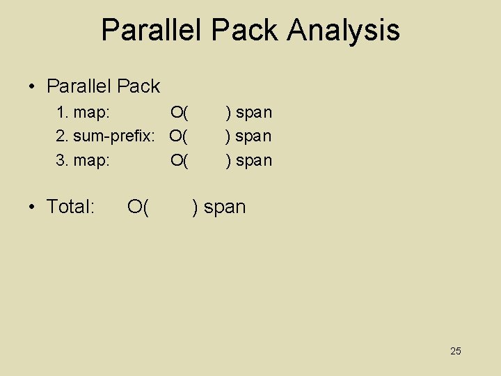
Parallel Pack Analysis • Parallel Pack 1. map: O( 2. sum-prefix: O( 3. map: O( • Total: O( ) span 25

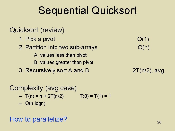
Sequential Quicksort (review): 1. Pick a pivot 2. Partition into two sub-arrays O(1) O(n) A. values less than pivot B. values greater than pivot 3. Recursively sort A and B 2 T(n/2), avg Complexity (avg case) – T(n) = n + 2 T(n/2) – O(n logn) How to parallelize? T(0) = T(1) = 1 26

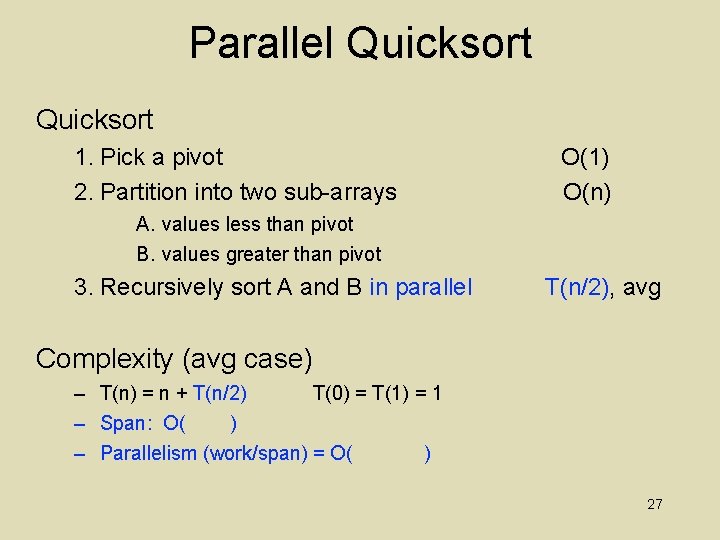
Parallel Quicksort 1. Pick a pivot 2. Partition into two sub-arrays O(1) O(n) A. values less than pivot B. values greater than pivot 3. Recursively sort A and B in parallel T(n/2), avg Complexity (avg case) – T(n) = n + T(n/2) T(0) = T(1) = 1 – Span: O( ) – Parallelism (work/span) = O( ) 27

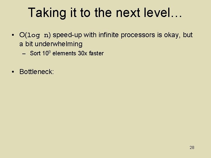
Taking it to the next level… • O(log n) speed-up with infinite processors is okay, but a bit underwhelming – Sort 109 elements 30 x faster • Bottleneck: 28

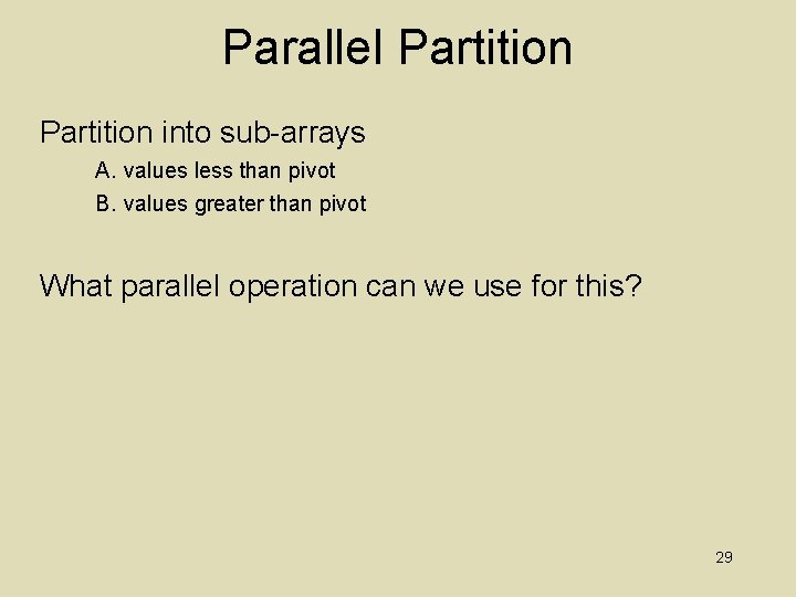
Parallel Partition into sub-arrays A. values less than pivot B. values greater than pivot What parallel operation can we use for this? 29

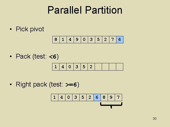
Parallel Partition • Pick pivot 8 1 4 9 0 3 5 2 7 6 • Pack (test: <6) 1 4 0 3 5 2 • Right pack (test: >=6) 1 4 0 3 5 2 6 8 9 7 30

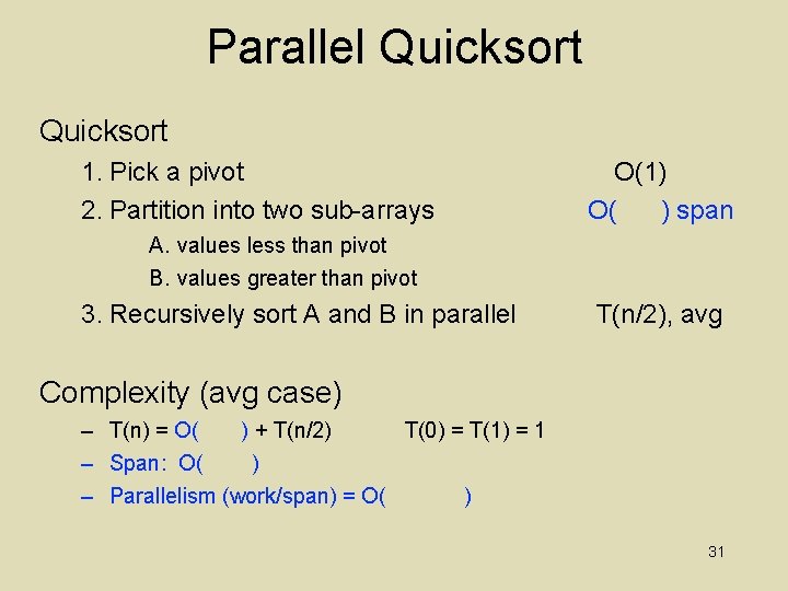
Parallel Quicksort 1. Pick a pivot 2. Partition into two sub-arrays O(1) O( ) span A. values less than pivot B. values greater than pivot 3. Recursively sort A and B in parallel T(n/2), avg Complexity (avg case) – T(n) = O( ) + T(n/2) T(0) = T(1) = 1 – Span: O( ) – Parallelism (work/span) = O( ) 31

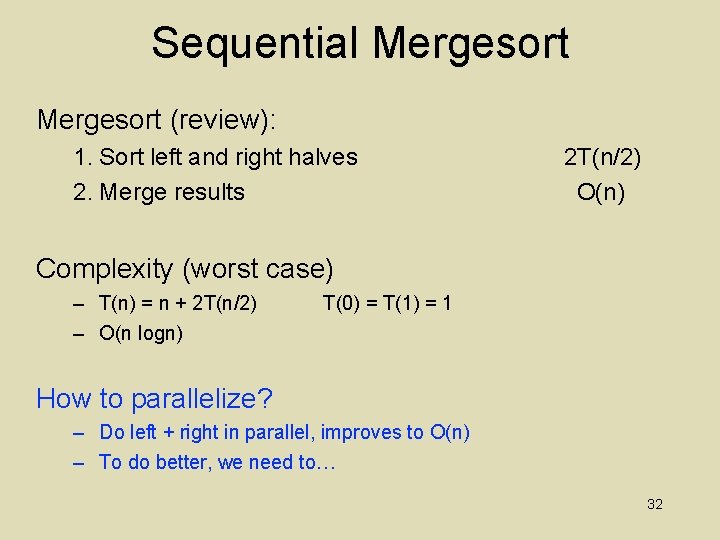
Sequential Mergesort (review): 1. Sort left and right halves 2. Merge results 2 T(n/2) O(n) Complexity (worst case) – T(n) = n + 2 T(n/2) – O(n logn) T(0) = T(1) = 1 How to parallelize? – Do left + right in parallel, improves to O(n) – To do better, we need to… 32

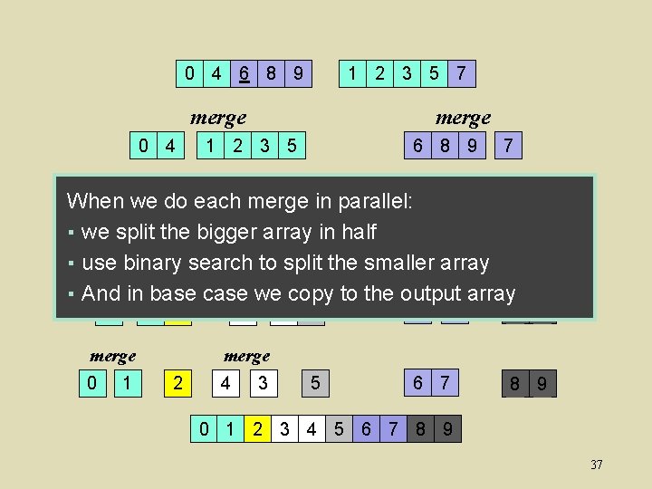
Parallel Merge 0 4 6 8 9 1 2 3 5 7 How to merge two sorted lists in parallel? 33

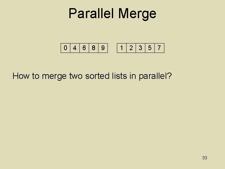
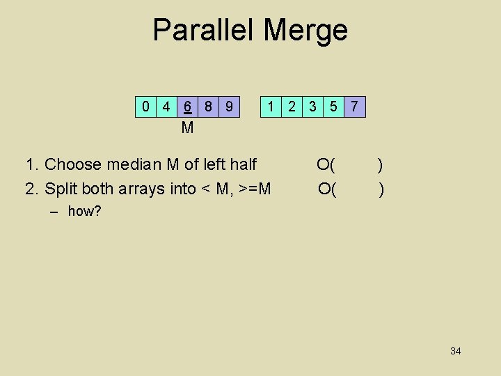
Parallel Merge 0 4 6 8 9 1 2 3 5 7 M 1. Choose median M of left half 2. Split both arrays into < M, >=M O( O( ) ) – how? 34

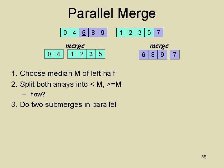
Parallel Merge 0 4 6 8 9 1 2 3 5 7 merge 0 4 1 2 3 5 merge 6 8 9 7 1. Choose median M of left half 2. Split both arrays into < M, >=M – how? 3. Do two submerges in parallel 35

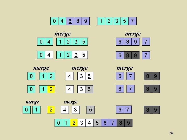
0 4 6 8 9 1 2 3 5 7 merge 0 4 1 2 3 5 6 8 9 7 merge 0 1 2 4 3 5 6 7 8 9 merge 0 merge 1 merge 2 4 3 5 6 7 8 9 0 1 2 3 4 5 6 7 8 9 36

0 4 6 8 9 1 2 3 5 7 merge 0 4 merge 1 2 3 5 6 8 9 7 0 4 1 2 3 5 When we do each merge in parallel: 6 8 9 7 ▪ we split the biggermerge array in half merge ▪ use 6 array 7 0 binary 1 2 search 4 to 3 split 5 the smaller 8 9 ▪ And in base case we copy to the output array 0 1 2 merge 0 1 4 3 5 6 7 8 9 merge 2 4 3 5 6 7 8 9 0 1 2 3 4 5 6 7 8 9 37

Parallel Mergesort Pseudocode Merge(arr[], left 1, left 2, right 1, right 2, out[], out 1, out 2 ) int left. Size = left 2 – left 1 int right. Size = right 2 – right 1 // Assert: out 2 – out 1 = left. Size + right. Size // We will assume left. Size > right. Size without loss of generality if (left. Size + right. Size < CUTOFF) sequential merge and copy into out[out 1. . out 2] int mid = (left 2 – left 1)/2 binary. Search arr[right 1. . right 2] to find j such that arr[j] ≤ arr[mid] ≤ arr[j+1] Merge(arr[], left 1, mid, right 1, j, out[], out 1+mid+j) Merge(arr[], mid+1, left 2, j+1, right 2, out[], out 1+mid+j+1, out 2) 38

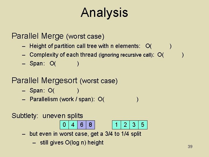
Analysis Parallel Merge (worst case) – Height of partition call tree with n elements: O( ) – Complexity of each thread (ignoring recursive call): O( – Span: O( ) ) Parallel Mergesort (worst case) – Span: O( ) – Parallelism (work / span): O( ) Subtlety: uneven splits 0 4 6 8 1 2 3 5 – but even in worst case, get a 3/4 to 1/4 split – still gives O(log n) height 39

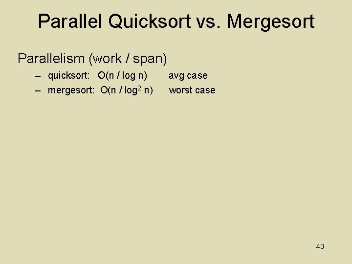
Parallel Quicksort vs. Mergesort Parallelism (work / span) – quicksort: O(n / log n) – mergesort: O(n / log 2 n) avg case worst case 40