CSE 291 Advanced Topics in Computational Biology L

CSE 291: Advanced Topics in Computational Biology L 3: population sub-structure/ admixture mapping Vineet Bafna/Pavel Pevzner www. cse. ucsd. edu/classes/sp 05/cse 291 -a

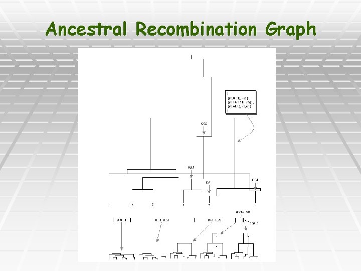
Ancestral Recombination Graph

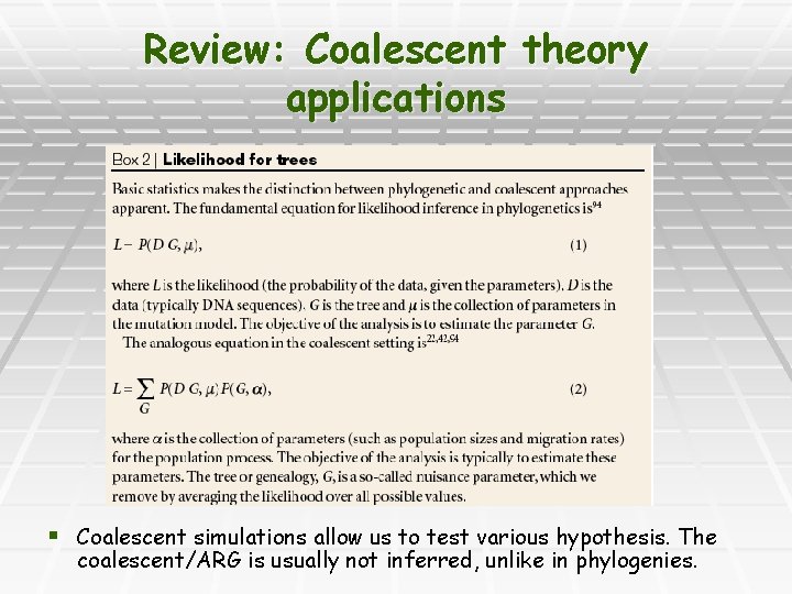
Review: Coalescent theory applications § Coalescent simulations allow us to test various hypothesis. The coalescent/ARG is usually not inferred, unlike in phylogenies.

Coalescent theory: example § Ex: ~1400 bp at Sod locus in Dros. § § § 10 taxa 5 were identical. The other 5 had 55 mutations. Q: Is this a chance event, or is there selection for this haplotype.

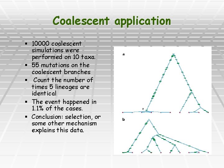
Coalescent application § 10000 coalescent simulations were performed on 10 taxa. § 55 mutations on the coalescent branches § Count the number of times 5 lineages are identical § The event happened in 1. 1% of the cases. § Conclusion: selection, or some other mechanism explains this data.

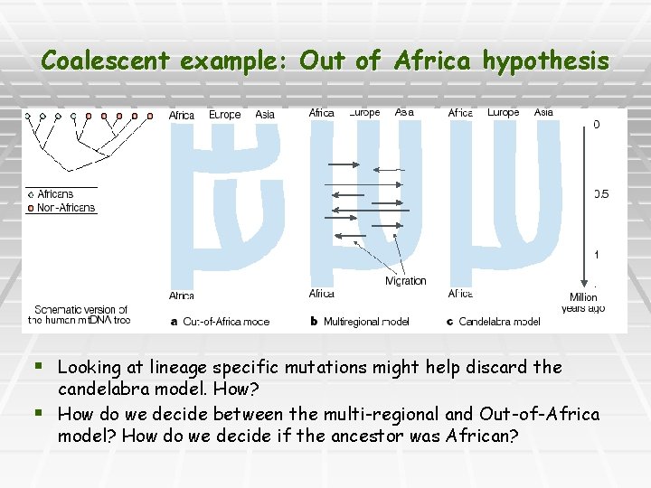
Coalescent example: Out of Africa hypothesis § Looking at lineage specific mutations might help discard the candelabra model. How? § How do we decide between the multi-regional and Out-of-Africa model? How do we decide if the ancestor was African?

Coalescent simulation § Example 2: § Sample from a region. What is the recombination rate in this region? § Gabriel et al. Science 2002. § 3 populations were sampled at multiple regions spanning the genome § 54 regions (Average size 250 Kb) § SNP density 1 over 2 Kb § 90 Individuals from Nigeria (Yoruban) § 93 Europeans § 42 Asian § 50 African American

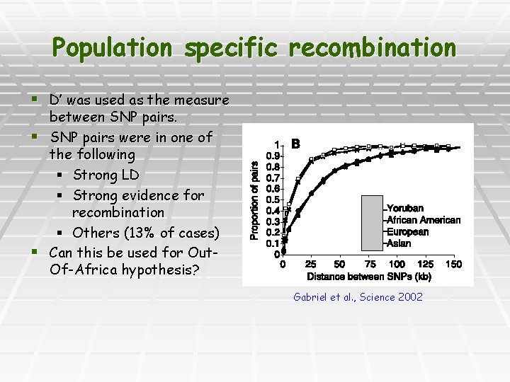
Population specific recombination § D’ was used as the measure between SNP pairs. § SNP pairs were in one of the following § Strong LD § Strong evidence for recombination § Others (13% of cases) § Can this be used for Out. Of-Africa hypothesis? Gabriel et al. , Science 2002

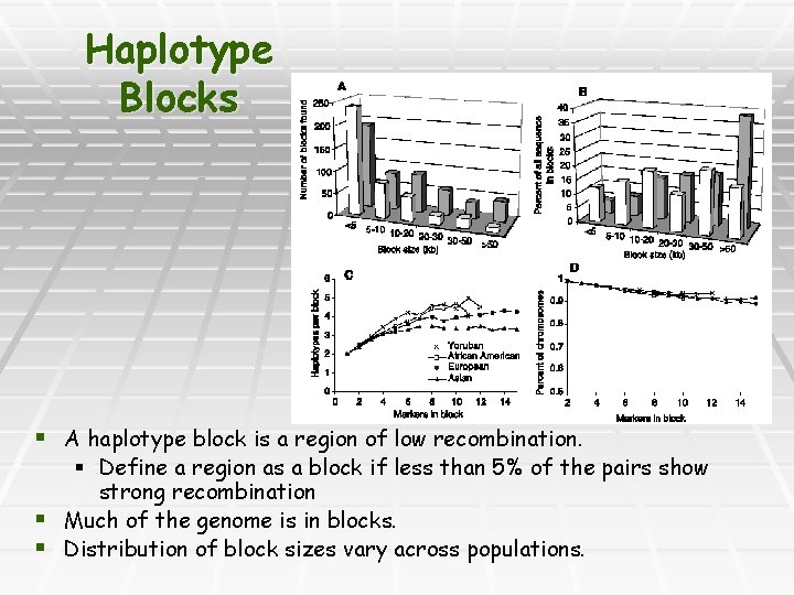
Haplotype Blocks § A haplotype block is a region of low recombination. § Define a region as a block if less than 5% of the pairs show strong recombination § Much of the genome is in blocks. § Distribution of block sizes vary across populations.

Testing Out-of-Africa § Generate simulations with and without migration. § Check size of haplotype blocks. § Does it vary when migrations are allowed? § When the ‘new’ population has a bottleneck? § If there were a bottleneck that created European and Asian populations, can we say anything about frequency of alleles that are ‘African specific’? § Should they be high frequency, or low frequency in African populations?

Haplotype Block: implications § The genome is mostly partitioned into haplotype blocks. § Within a block, there is extensive LD. § Is this good, or bad, for association mapping?

Population Sub-structure

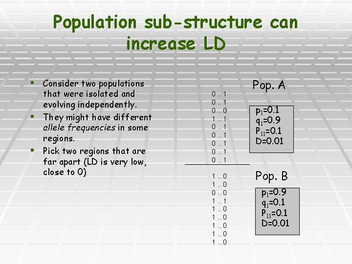
Population sub-structure can increase LD § Consider two populations that were isolated and evolving independently. § They might have different allele frequencies in some regions. § Pick two regions that are far apart (LD is very low, close to 0) 0. . 1 0. . 0 1. . 1 0. . 1 1. . 0 0. . 0 1. . 1 1. . 0 Pop. A p 1=0. 1 q 1=0. 9 P 11=0. 1 D=0. 01 Pop. B p 1=0. 9 q 1=0. 1 P 11=0. 1 D=0. 01

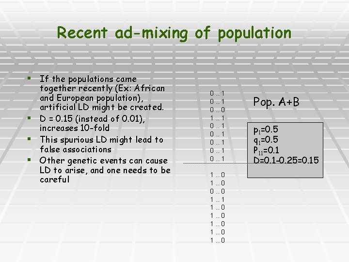
Recent ad-mixing of population § If the populations came together recently (Ex: African and European population), artificial LD might be created. § D = 0. 15 (instead of 0. 01), increases 10 -fold § This spurious LD might lead to false associations § Other genetic events can cause LD to arise, and one needs to be careful 0. . 1 0. . 0 1. . 1 0. . 1 1. . 0 0. . 0 1. . 1 1. . 0 Pop. A+B p 1=0. 5 q 1=0. 5 P 11=0. 1 D=0. 1 -0. 25=0. 15

Determining population substructure § Given a mix of people, can you sub-divide them into ethnic populations. § Turn the ‘problem’ of spurious LD into a clue. § Find markers that are too far apart to show LD § If they do show LD (correlation), that shows the existence of multiple populations. § Sub-divide them into populations so that LD disappears.

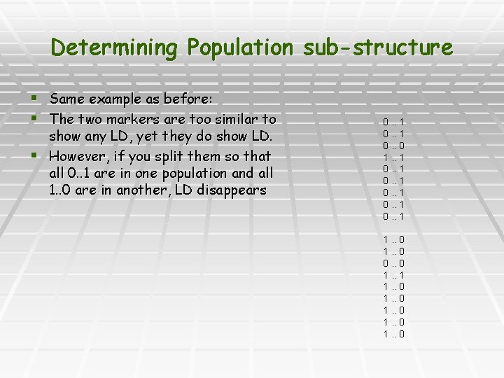
Determining Population sub-structure § Same example as before: § The two markers are too similar to show any LD, yet they do show LD. § However, if you split them so that all 0. . 1 are in one population and all 1. . 0 are in another, LD disappears 0. . 1 0. . 0 1. . 1 0. . 1 1. . 0 0. . 0 1. . 1 1. . 0

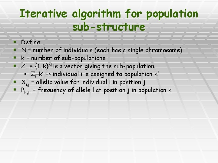
Iterative algorithm for population sub-structure Define N = number of individuals (each has a single chromosome) k = number of sub-populations. Z {1. . k}N is a vector giving the sub-population. § Zi=k’ => individual i is assigned to population k’ § Xi, j = allelic value for individual i in position j § Pk, j, l = frequency of allele l at position j in population k § §

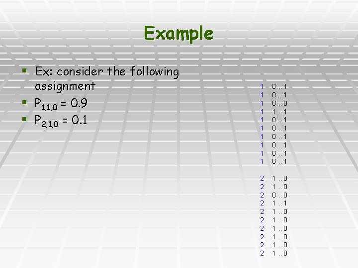
Example § Ex: consider the following assignment § P 1, 1, 0 = 0. 9 § P 2, 1, 0 = 0. 1 1 1 0. . 0 1. . 1 0. . 1 2 2 2 2 2 1. . 0 0. . 0 1. . 1 1. . 0

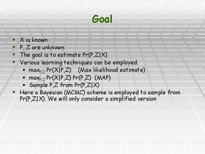
Goal X is known. P, Z are unknown. The goal is to estimate Pr(P, Z|X) Various learning techniques can be employed. § max. P, Z Pr(X|P, Z) (Max likelihood estimate) § max. P, Z Pr(X|P, Z) Pr(P, Z) (MAP) § Sample P, Z from Pr(P, Z|X) § Here a Bayesian (MCMC) scheme is employed to sample from Pr(P, Z|X). We will only consider a simplified version § §

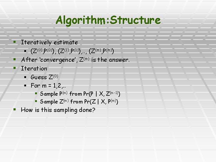
Algorithm: Structure § Iteratively estimate § (Z(0), P(0)), (Z(1), P(1)), . . , (Z(m), P(m)) § After ‘convergence’, Z(m) is the answer. § Iteration § Guess Z(0) § For m = 1, 2, . . § Sample P(m) from Pr(P | X, Z(m-1)) § Sample Z(m) from Pr(Z | X, P(m)) § How is this sampling done?

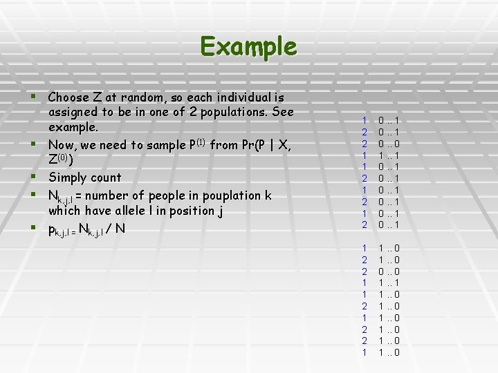
Example § Choose Z at random, so each individual is § § assigned to be in one of 2 populations. See example. Now, we need to sample P(1) from Pr(P | X, Z(0)) Simply count Nk, j, l = number of people in pouplation k which have allele l in position j pk, j, l = Nk, j, l / N 1 2 2 1 1 2 1 2 0. . 1 0. . 0 1. . 1 0. . 1 1 2 2 1 1. . 0 0. . 0 1. . 1 1. . 0

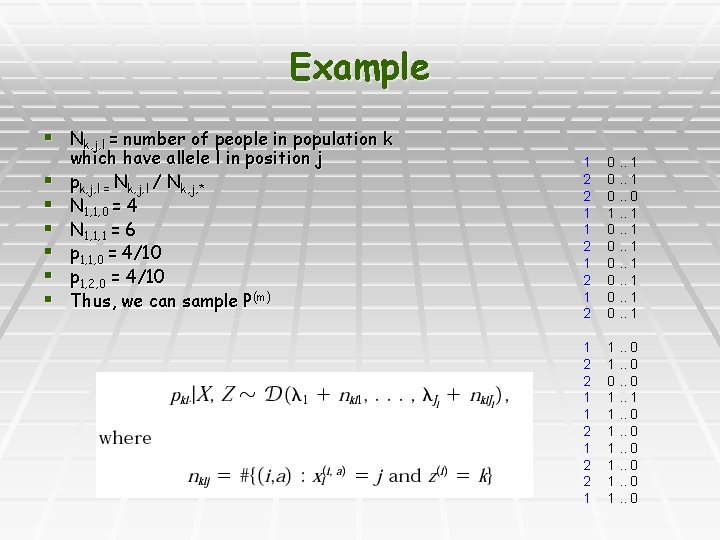
Example § Nk, j, l = number of people in population k § § § which have allele l in position j pk, j, l = Nk, j, l / Nk, j, * N 1, 1, 0 = 4 N 1, 1, 1 = 6 p 1, 1, 0 = 4/10 p 1, 2, 0 = 4/10 Thus, we can sample P(m) 1 2 2 1 1 2 1 2 0. . 1 0. . 0 1. . 1 0. . 1 1 2 2 1 1. . 0 0. . 0 1. . 1 1. . 0

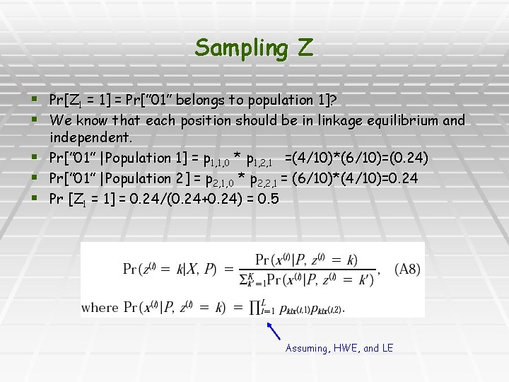
Sampling Z § Pr[Z 1 = 1] = Pr[” 01” belongs to population 1]? § We know that each position should be in linkage equilibrium and § § § independent. Pr[” 01” |Population 1] = p 1, 1, 0 * p 1, 2, 1 =(4/10)*(6/10)=(0. 24) Pr[” 01” |Population 2] = p 2, 1, 0 * p 2, 2, 1 = (6/10)*(4/10)=0. 24 Pr [Z 1 = 1] = 0. 24/(0. 24+0. 24) = 0. 5 Assuming, HWE, and LE

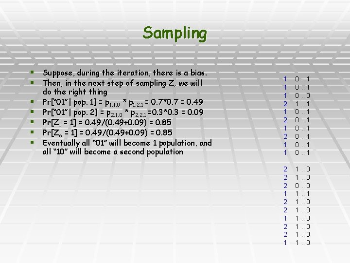
Sampling § Suppose, during the iteration, there is a bias. § Then, in the next step of sampling Z, we will § § § do the right thing Pr[“ 01”| pop. 1] = p 1, 1, 0 * p 1, 2, 1 = 0. 7*0. 7 = 0. 49 Pr[“ 01”| pop. 2] = p 2, 1, 0 * p 2, 2, 1 =0. 3*0. 3 = 0. 09 Pr[Z 1 = 1] = 0. 49/(0. 49+0. 09) = 0. 85 Pr[Z 6 = 1] = 0. 49/(0. 49+0. 09) = 0. 85 Eventually all “ 01” will become 1 population, and all “ 10” will become a second population 1 1 1 2 1 2 1 1 0. . 0 1. . 1 0. . 1 2 2 2 1 1. . 0 0. . 0 1. . 1 1. . 0

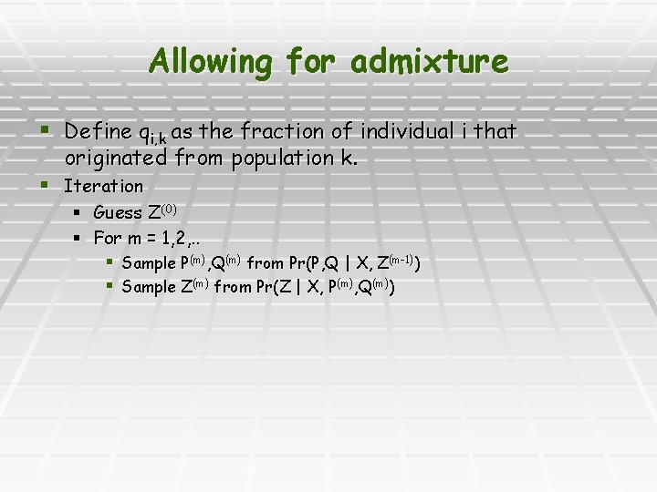
Allowing for admixture § Define qi, k as the fraction of individual i that originated from population k. § Iteration § Guess Z(0) § For m = 1, 2, . . § Sample P(m), Q(m) from Pr(P, Q | X, Z(m-1)) § Sample Z(m) from Pr(Z | X, P(m), Q(m))

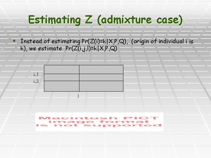
Estimating Z (admixture case) § Instead of estimating Pr(Z(i)=k|X, P, Q), (origin of individual i is k), we estimate Pr(Z(i, j, l)=k|X, P, Q) i, 1 i, 2 j

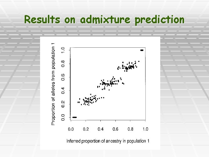
Results on admixture prediction

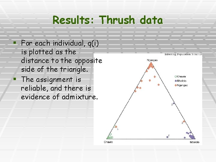
Results: Thrush data § For each individual, q(i) is plotted as the distance to the opposite side of the triangle. § The assignment is reliable, and there is evidence of admixture.

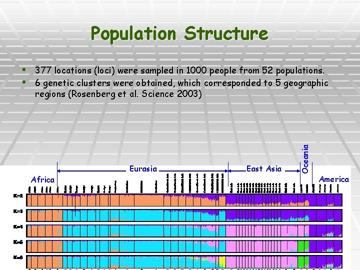
Population Structure § 377 locations (loci) were sampled in 1000 people from 52 populations. § 6 genetic clusters were obtained, which corresponded to 5 geographic Africa Eurasia East Asia Oceania regions (Rosenberg et al. Science 2003) America

Population sub-structure: research problem § Systematically explore the effect of admixture. Can admixture be predicted for a locus, or for an individual § The sampling approach may or may not be appropriate. Formulate as an optimization/learning problem: § (w/out admixture). Assign individuals to sub-populations so as to maximize linkage equilibrium, and hardy weinberg equilibrium in each of the sub-populations § (w/ admixture) Assign (individuals, loci) to sub-populations

Admixture mapping