CSE 245 Computer Aided Circuit Simulation and Verification

CSE 245: Computer Aided Circuit Simulation and Verification Fall 2004, Nov Transmission Line Simulation 1/12/2022 1

Outline o o o Transmission Line Equations FDTD Solution of The Transmission Line Equations Convolution Simulation of Transmission Lines 12 January 2022 2

Lumped V. S. Distributed Circuits o Lumped circuit: n n n o In circuit theory, we assume the physical dimensions of a circuit element are much smaller than the electrical wavelength. Resistor, Capacitor, Inductor, Independent and dependent sources are lumped circuit elements The voltages and currents in such a circuit are functions of time only. Distributed Circuit: n n 1/12/2022 In a distributed circuit, for example in a transmission line circuit. The size of the transmission line may be a considerable fraction of a wavelength, or many wavelengths. Thus a transmission line can’t be modeled as a lumped circuit element. It should be modeled as a distributed parameter network, where voltages and currents are functions of position as well as time 3

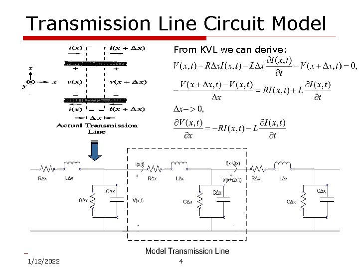
Transmission Line Circuit Model From KVL we can derive: 1/12/2022 4

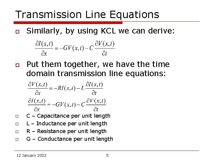
Transmission Line Equations o o o Similarly, by using KCL we can derive: Put them together, we have the time domain transmission line equations: C – Capacitance per unit length L – Inductance per unit length R – Resistance per unit length G – Conductance per unit length 12 January 2022 5

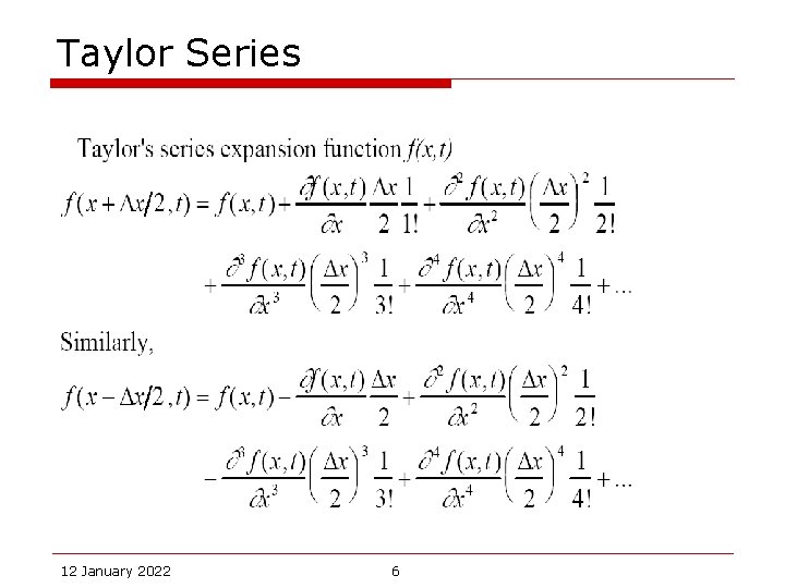
Taylor Series 12 January 2022 6

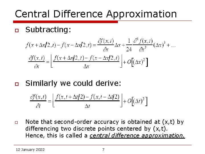
Central Difference Approximation o Subtracting: o Similarly we could derive: o Note that second-order accuracy is obtained at (x, t) by differencing two discrete points centered by (x, t). Hence, this is called a central difference approximation. 12 January 2022 7

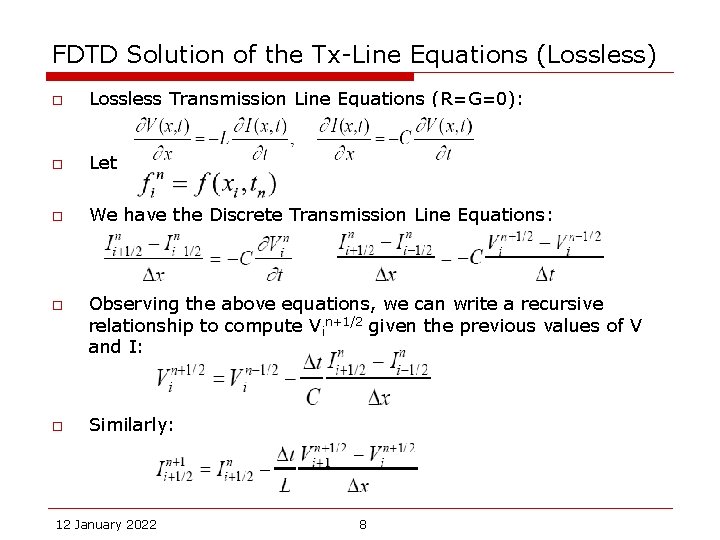
FDTD Solution of the Tx-Line Equations (Lossless) o Lossless Transmission Line Equations (R=G=0): o Let o We have the Discrete Transmission Line Equations: o o Observing the above equations, we can write a recursive relationship to compute Vin+1/2 given the previous values of V and I: Similarly: 12 January 2022 8

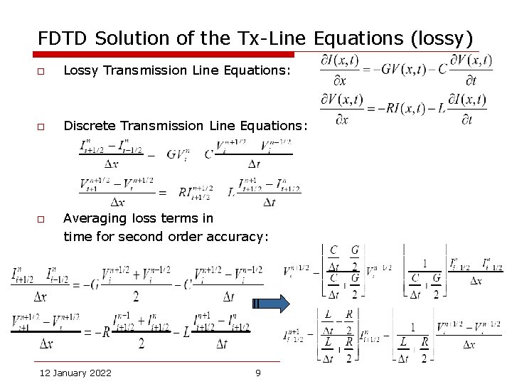
FDTD Solution of the Tx-Line Equations (lossy) o Lossy Transmission Line Equations: o Discrete Transmission Line Equations: o Averaging loss terms in time for second order accuracy: 12 January 2022 9

Summary: FDTD Solution of the Tx-Line Equations o FDTD Summary: n n Line axis x is discretized in Δx increments or spatial cells, the time variable t is discretized in Δt increments or temporal cells. The derivatives in the Tx-Line Equations are approximated by central differences. Given the initial condition of V and I along the entire line length, V and I can be time advanced. The accuracy of the solution depends on having sufficiently small spatial (Δx) and temporal (Δt) cell sizes 12 January 2022 10

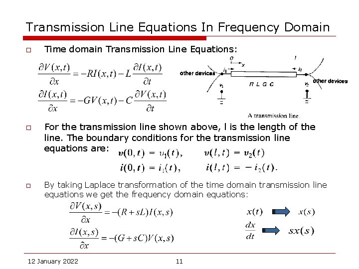
Transmission Line Equations In Frequency Domain o o o Time domain Transmission Line Equations: For the transmission line shown above, l is the length of the line. The boundary conditions for the transmission line equations are: By taking Laplace transformation of the time domain transmission line equations we get the frequency domain equations: 12 January 2022 11

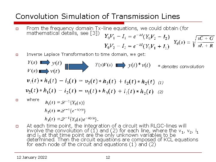
Convolution Simulation of Transmission Lines o o From the frequency domain Tx-line equations, we could obtain (for mathematical details, see [3]) Inverse Laplace Transformation to time domain, we get: * denotes convolution (1) (2) o o where At each time point, the integration of a circuit with RLGC-lines will involve the convolution of (1) and (2) for each line, where the v 1, v 2, i 1 and i 2 at that time point are the only unknown variables to be determined. Then the circuit equations are composed of KCL equations for each node of the circuit and equations (1) and (2) 12 January 2022 12

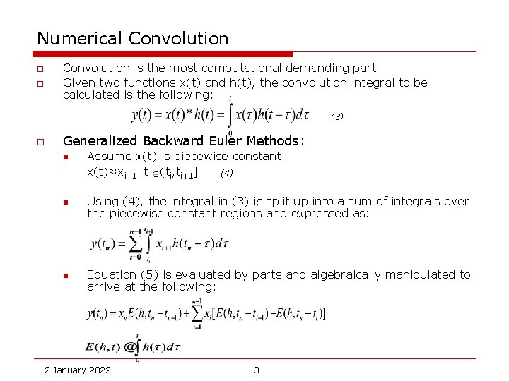
Numerical Convolution o o Convolution is the most computational demanding part. Given two functions x(t) and h(t), the convolution integral to be calculated is the following: (3) o Generalized Backward Euler Methods: n n n Assume x(t) is piecewise constant: x(t)≈xi+1, t (ti, ti+1] (4) Using (4), the integral in (3) is split up into a sum of integrals over the piecewise constant regions and expressed as: Equation (5) is evaluated by parts and algebraically manipulated to arrive at the following: 12 January 2022 13

Numerical Convolution o o If we assume x(t)≈xi, t [ti, ti+1), a generalized forward Euler method could be derived. Similarly, by assuming x(t) is piecewise linear we could derive the generalized trapezoidal convolution method. For details, see [3] 12 January 2022 14

References: o o [1] Finite-difference, time-domain analysis of lossy transmission lines, Roden, J. A. Paul, C. R. Smith, W. T. Gedney, S. D. IEEE Transactions on Electromagnetic Compatibility, Feb 1996 [2] EE 669 class notes, Stephen Gedney, University of Kentucky [3] Algorithms for the Transient Simulation of Lossy Interconnect. J. S. Roychowdhury, A. R. Newton, D. O. Pederson. IEEE Transactions on Computer-Aided Design of Integrated Circuits and Systems. Vol. 13, No. 1. Jan 1994 [4] Transient Simulation of Lossy Interconnects Based on the Recursive Convolution Formulation, S. Lin and E. S. Kuh, IEEE Transactions on Circuits and Systems – I, Vol. 39, No. 11, Nov 1992 12 January 2022 15