CSE 233 Course Review CSE POSTECH What we

CSE 233 Course Review CSE, POSTECH

What we studied in the 1 st half Week 1 : Overview of C++, Program performance Week 2 : Array-based and linked representations of Lists Week 3 : Arrays and Matrices Week 4 : Performance Measurement Week 5 : Stacks Week 6 : Queues Week 7 : Skip lists and Hashing Week 8 : Review and Midterm Exam

What we studied in the 2 nd half Week 9 : Binary and other trees Week 10 : Priority queues, Heaps, Leftist trees Week 11 : Tournament trees and Bin packing Week 12 : Binary search trees Week 13 : AVL trees Week 14 : Graphs Week 15 : Graph Search Methods Week 16 : Review and Final exam

Trees

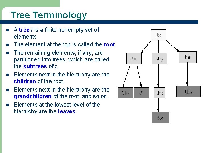
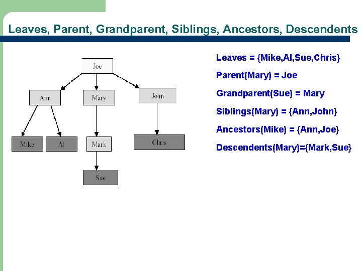
Tree Terminology l l l A tree t is a finite nonempty set of elements The element at the top is called the root The remaining elements, if any, are partitioned into trees, which are called the subtrees of t. Elements next in the hierarchy are the children of the root. Elements next in the hierarchy are the grandchildren of the root, and so on. Elements at the lowest level of the hierarchy are the leaves.

Leaves, Parent, Grandparent, Siblings, Ancestors, Descendents Leaves = {Mike, AI, Sue, Chris} Parent(Mary) = Joe Grandparent(Sue) = Mary Siblings(Mary) = {Ann, John} Ancestors(Mike) = {Ann, Joe} Descendents(Mary)={Mark, Sue}

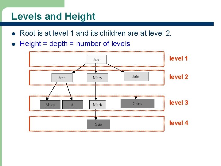
Levels and Height l l Root is at level 1 and its children are at level 2. Height = depth = number of levels level 1 level 2 level 3 level 4

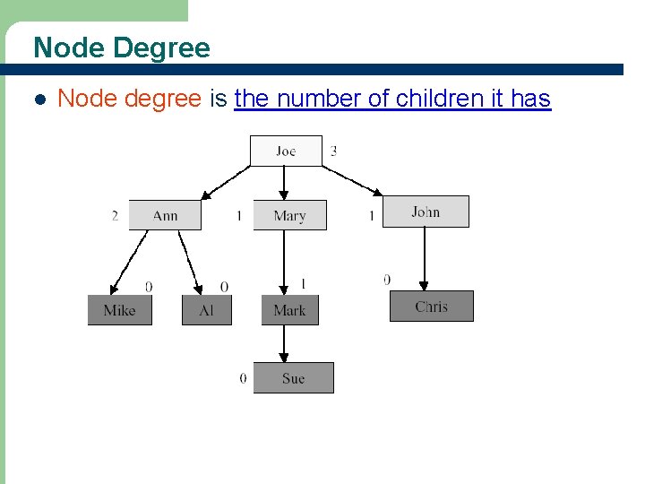
Node Degree l Node degree is the number of children it has

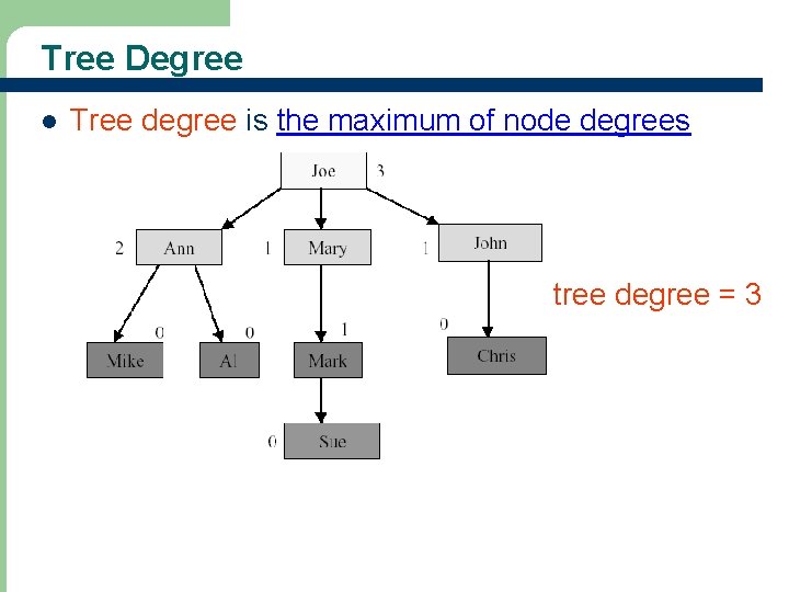
Tree Degree l Tree degree is the maximum of node degrees tree degree = 3

Binary Trees

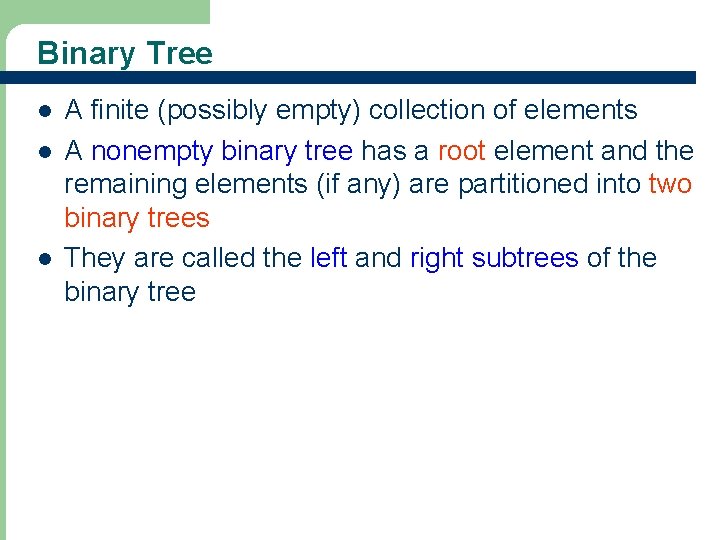
Binary Tree l l l A finite (possibly empty) collection of elements A nonempty binary tree has a root element and the remaining elements (if any) are partitioned into two binary trees They are called the left and right subtrees of the binary tree

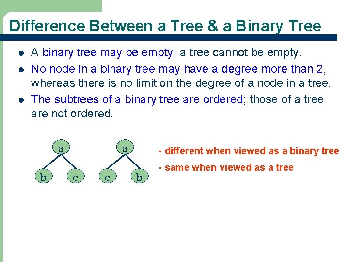
Difference Between a Tree & a Binary Tree l l l A binary tree may be empty; a tree cannot be empty. No node in a binary tree may have a degree more than 2, whereas there is no limit on the degree of a node in a tree. The subtrees of a binary tree are ordered; those of a tree are not ordered. a b a c c - different when viewed as a binary tree b - same when viewed as a tree

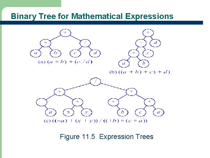
Binary Tree for Mathematical Expressions Figure 11. 5 Expression Trees

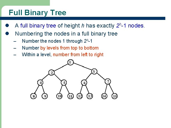
Full Binary Tree l A full binary tree of height h has exactly 2 h-1 nodes. l Numbering the nodes in a full binary tree – – – Number the nodes 1 through 2 h-1 Number by levels from top to bottom Within a level, number from left to right

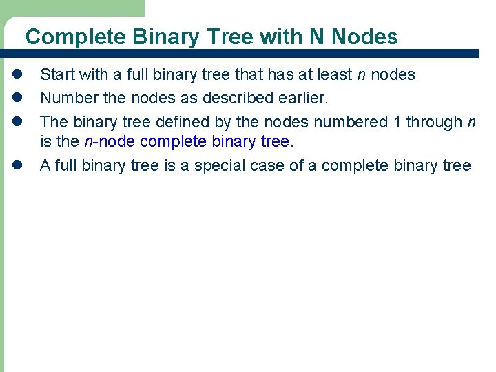
Complete Binary Tree with N Nodes l Start with a full binary tree that has at least n nodes l Number the nodes as described earlier. l The binary tree defined by the nodes numbered 1 through n is the n-node complete binary tree. l A full binary tree is a special case of a complete binary tree

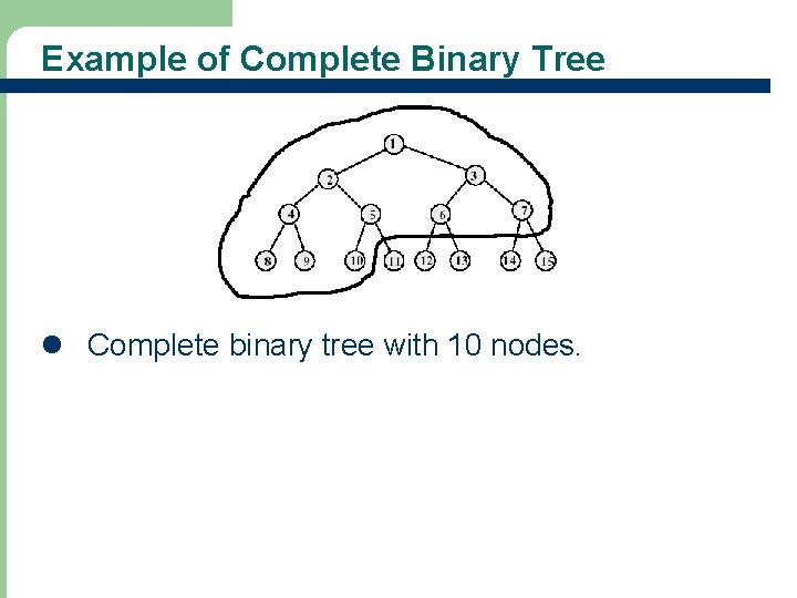
Example of Complete Binary Tree l Complete binary tree with 10 nodes.

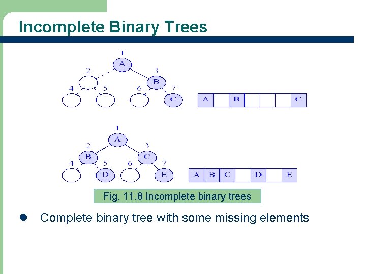
Incomplete Binary Trees Fig. 11. 8 Incomplete binary trees l Complete binary tree with some missing elements

Binary Tree Representation l Array representation l Linked representation

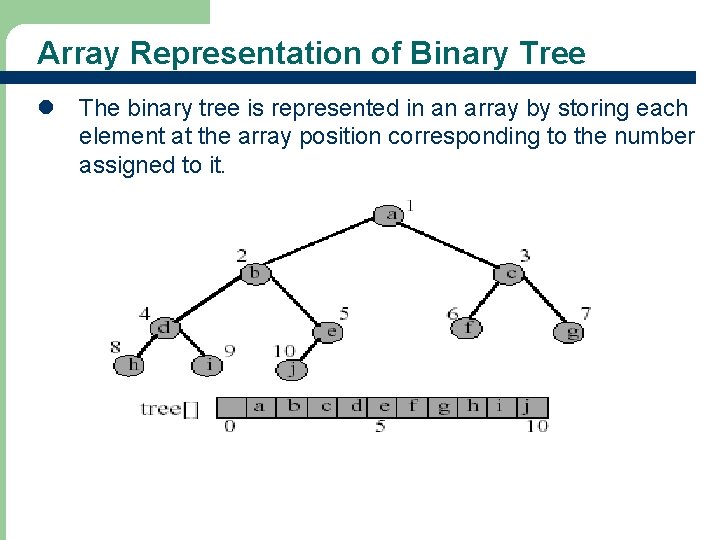
Array Representation of Binary Tree l The binary tree is represented in an array by storing each element at the array position corresponding to the number assigned to it.

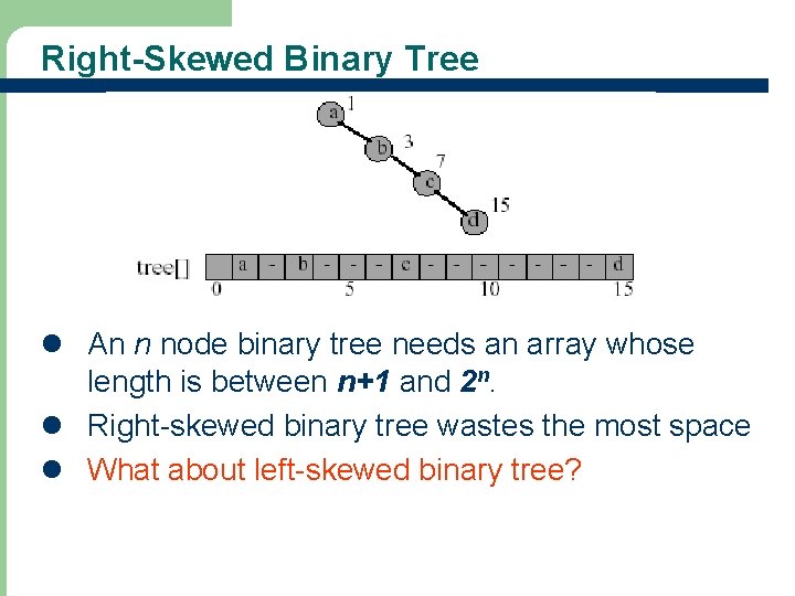
Right-Skewed Binary Tree l An n node binary tree needs an array whose length is between n+1 and 2 n. l Right-skewed binary tree wastes the most space l What about left-skewed binary tree?

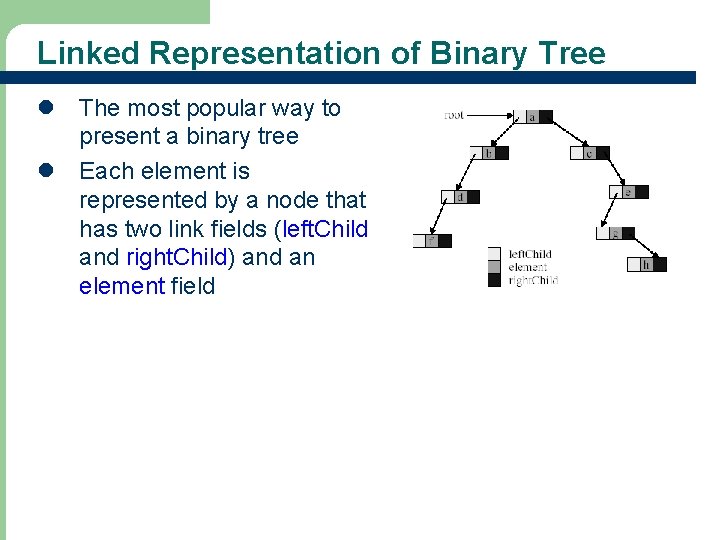
Linked Representation of Binary Tree l The most popular way to present a binary tree l Each element is represented by a node that has two link fields (left. Child and right. Child) and an element field

Priority Queues

Priority Queues l l l A priority queue is a collection of zero or more elements each element has a priority or value Unlike the FIFO queues, the order of deletion from a priority queue (e. g. , who gets served next) is determined by the element priority Elements are deleted by increasing or decreasing order of priority rather than by the order in which they arrived in the queue

Priority Queues l Operations performed on priority queues 1) Find an element, 2) insert a new element, 3) delete an element, etc. l l l In a Min priority queue, find/delete operation finds/deletes the element with minimum priority In a Max priority queue, find/delete operation finds/deletes the element with maximum priority Two or more elements can have the same priority

Implementation of Priority Queues l l l Implemented using heaps and leftist trees Heap is a complete binary tree that is efficiently stored using the array-based representation Leftist tree is a linked data structure suitable for the implementation of a priority queue

Min (Max) Trees

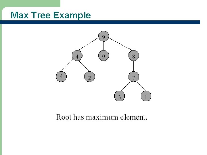
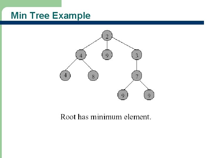
Max (Min) Tree l A max tree (min tree) is a tree in which the value in each node is greater (less) than or equal to those in its children (if any) – Nodes of a max or min tree may have more than two children (i. e. , may not be binary tree)

Max Tree Example

Min Tree Example

Heaps

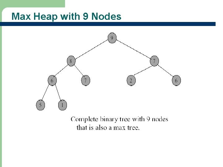
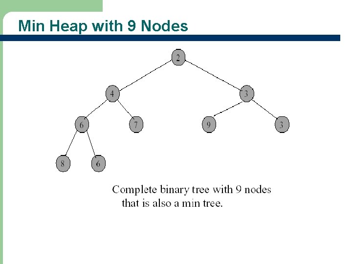
Heaps - Definitions l A max heap (min heap) is a max (min) tree that is also a complete binary tree

Max Heap with 9 Nodes

Min Heap with 9 Nodes

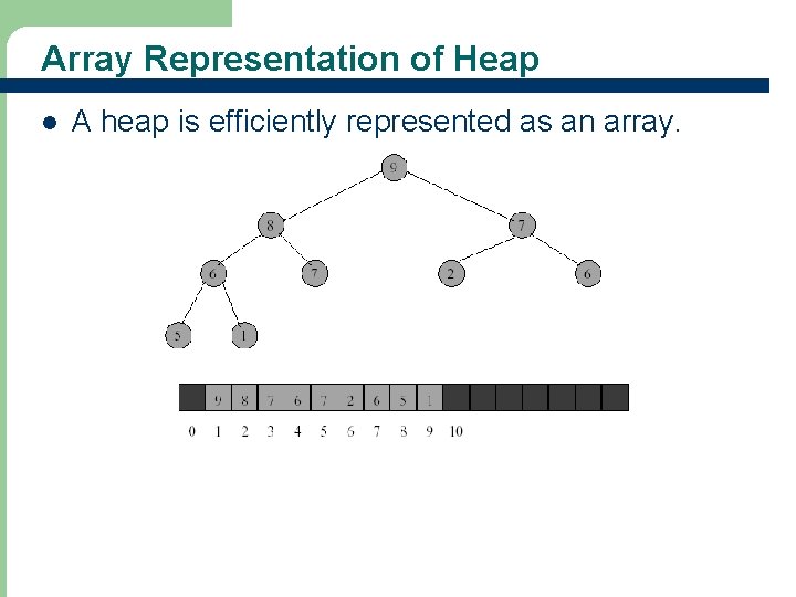
Array Representation of Heap l A heap is efficiently represented as an array.

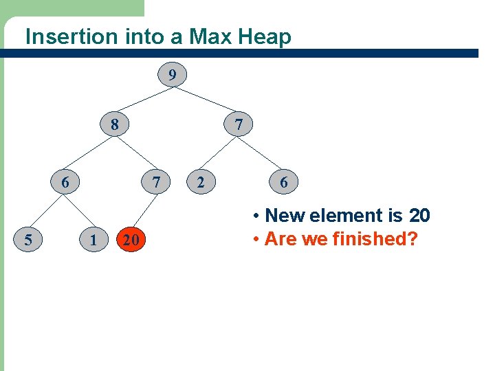
Insertion into a Max Heap 9 8 7 6 5 7 1 20 2 6 • New element is 20 • Are we finished?

Insertion into a Max Heap 9 8 7 6 5 20 1 7 2 6 • Exchange the positions with 7 • Are we finished?

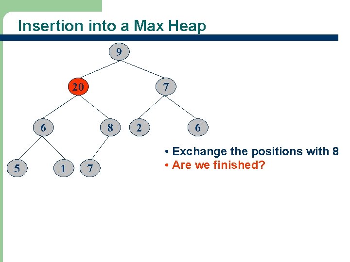
Insertion into a Max Heap 9 20 7 6 5 8 1 7 2 6 • Exchange the positions with 8 • Are we finished?

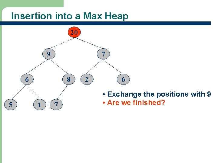
Insertion into a Max Heap 20 9 7 6 5 8 1 7 2 6 • Exchange the positions with 9 • Are we finished?

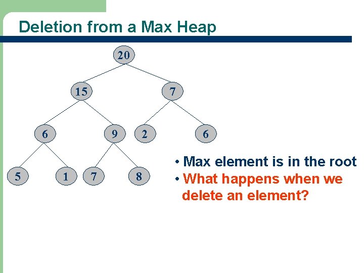
Deletion from a Max Heap 20 15 7 6 5 9 1 7 2 8 6 • Max element is in the root • What happens when we delete an element?

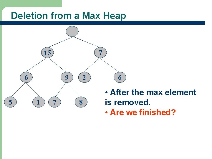
Deletion from a Max Heap 15 7 6 5 9 1 7 2 8 6 • After the max element is removed. • Are we finished?

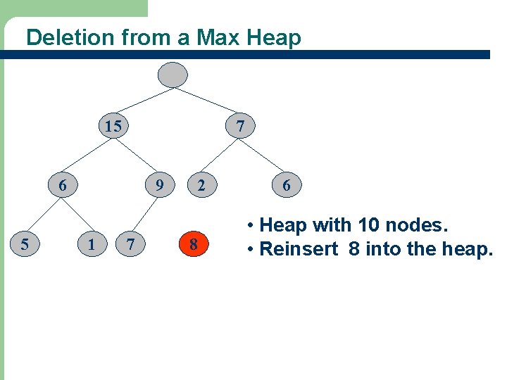
Deletion from a Max Heap 15 7 6 5 9 1 7 2 8 6 • Heap with 10 nodes. • Reinsert 8 into the heap.

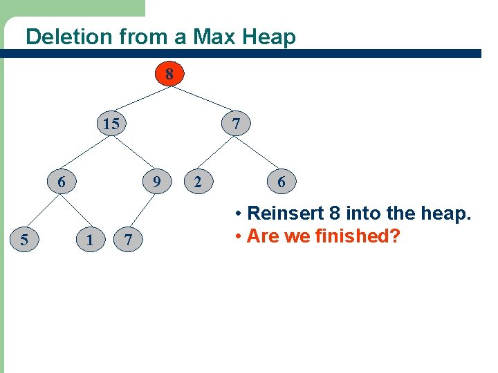
Deletion from a Max Heap 8 15 7 6 5 9 1 7 2 6 • Reinsert 8 into the heap. • Are we finished?

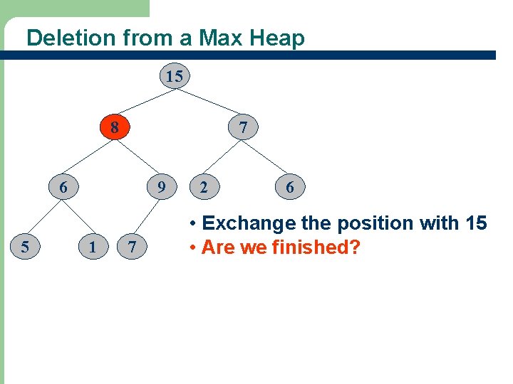
Deletion from a Max Heap 15 8 7 6 5 9 1 7 2 6 • Exchange the position with 15 • Are we finished?

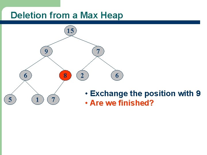
Deletion from a Max Heap 15 9 7 6 5 8 1 7 2 6 • Exchange the position with 9 • Are we finished?

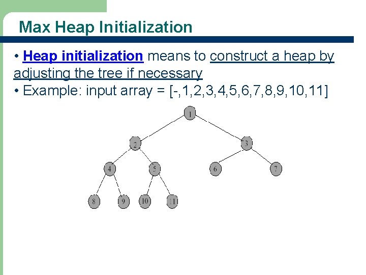
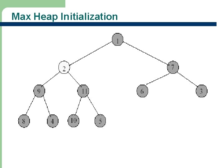
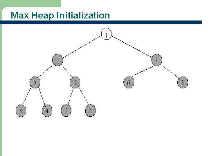
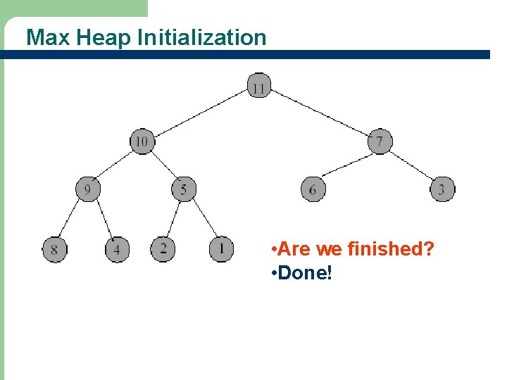
Max Heap Initialization • Heap initialization means to construct a heap by adjusting the tree if necessary • Example: input array = [-, 1, 2, 3, 4, 5, 6, 7, 8, 9, 10, 11]

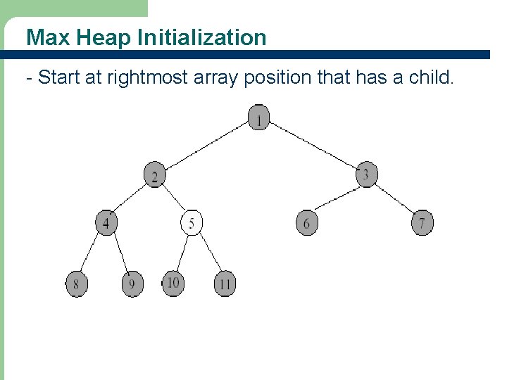
Max Heap Initialization - Start at rightmost array position that has a child.

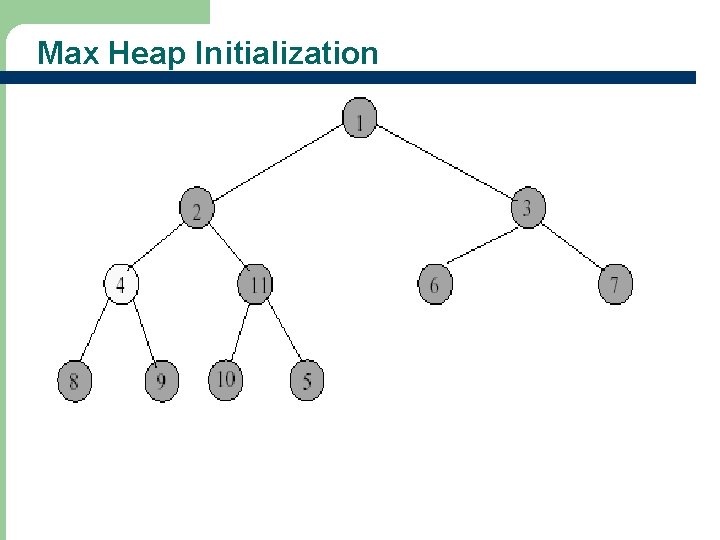
Max Heap Initialization

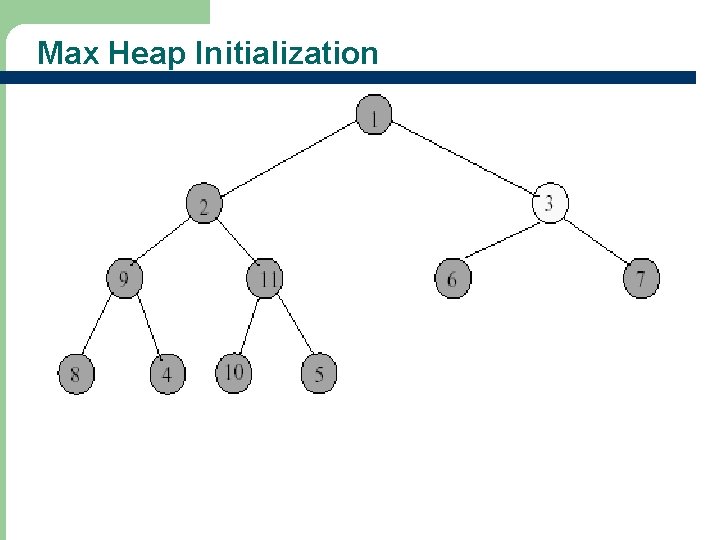
Max Heap Initialization

Max Heap Initialization

Max Heap Initialization

Max Heap Initialization • Are we finished? • Done!

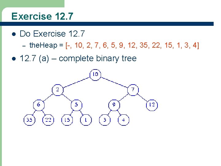
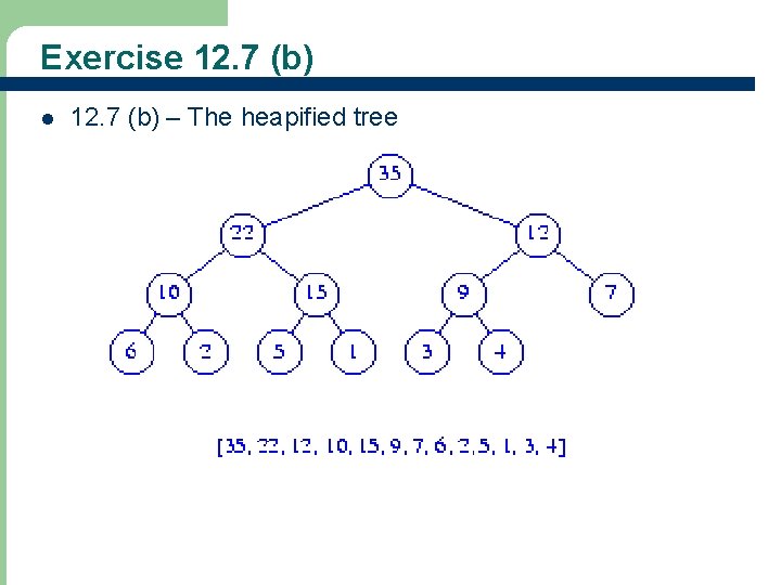
Exercise 12. 7 l Do Exercise 12. 7 – l the. Heap = [-, 10, 2, 7, 6, 5, 9, 12, 35, 22, 15, 1, 3, 4] 12. 7 (a) – complete binary tree

Exercise 12. 7 (b) l 12. 7 (b) – The heapified tree

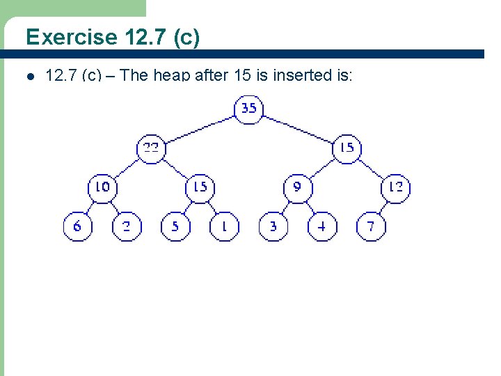
Exercise 12. 7 (c) l 12. 7 (c) – The heap after 15 is inserted is:

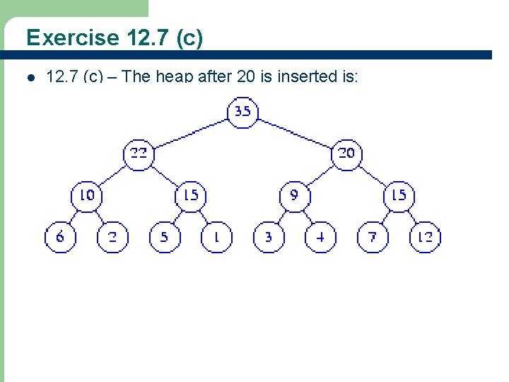
Exercise 12. 7 (c) l 12. 7 (c) – The heap after 20 is inserted is:

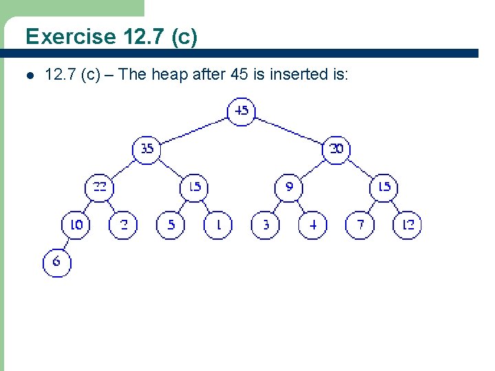
Exercise 12. 7 (c) l 12. 7 (c) – The heap after 45 is inserted is:

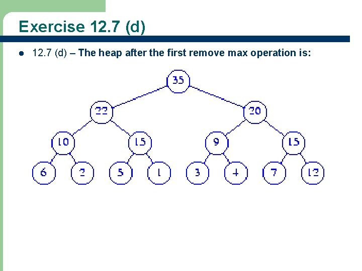
Exercise 12. 7 (d) l 12. 7 (d) – The heap after the first remove max operation is:

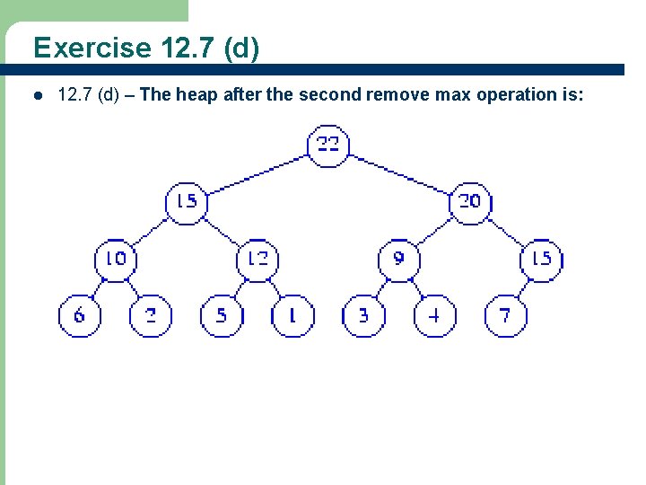
Exercise 12. 7 (d) l 12. 7 (d) – The heap after the second remove max operation is:

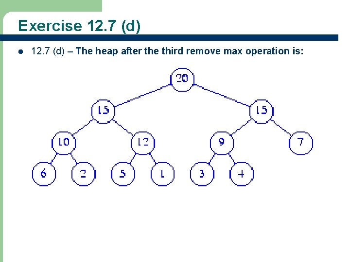
Exercise 12. 7 (d) l 12. 7 (d) – The heap after the third remove max operation is:

Leftist Trees

Leftist Trees l l l Leftist tree is a tree which tends to lean to the left Leftist tree structures are useful for applications – to meld (i. e. , combine) pairs of priority queues – using multiple queues of varying size External node – a special node that replaces each empty subtree Internal node – a node with non-empty subtrees Extended binary tree – a binary tree with external nodes added

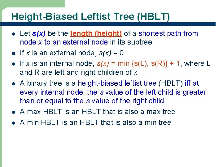
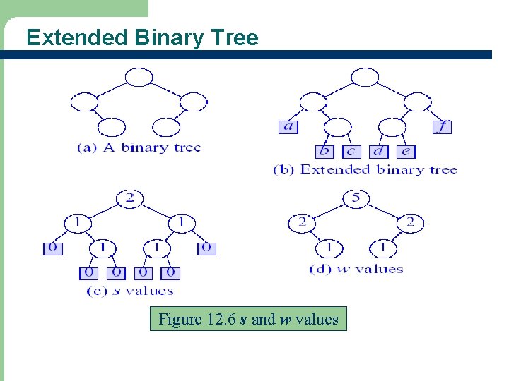
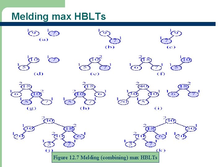
Height-Biased Leftist Tree (HBLT) l l l Let s(x) be the length (height) of a shortest path from node x to an external node in its subtree If x is an external node, s(x) = 0 If x is an internal node, s(x) = min {s(L), s(R)} + 1, where L and R are left and right children of x A binary tree is a height-biased leftist tree (HBLT) iff at every internal node, the s value of the left child is greater than or equal to the s value of the right child A max HBLT is an HBLT that is also a max tree A min HBLT is an HBLT that is also a min tree

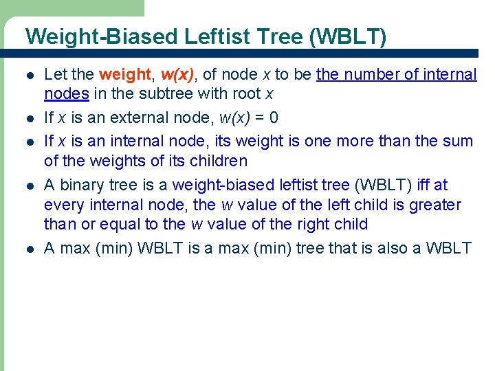
Weight-Biased Leftist Tree (WBLT) l l l Let the weight, w(x), of node x to be the number of internal nodes in the subtree with root x If x is an external node, w(x) = 0 If x is an internal node, its weight is one more than the sum of the weights of its children A binary tree is a weight-biased leftist tree (WBLT) iff at every internal node, the w value of the left child is greater than or equal to the w value of the right child A max (min) WBLT is a max (min) tree that is also a WBLT

Extended Binary Tree Figure 12. 6 s and w values

Melding max HBLTs Figure 12. 7 Melding (combining) max HBLTs

Applications of Heaps l l l Sort (heap sort) Machine scheduling Huffman codes

Heap Sort use element key as priority Algorithm l put elements to be sorted into a priority queue (i. e. , initialize a heap) l extract (delete) elements from the priority queue l – – if a min priority queue is used, elements are extracted in non-decreasing order of priority if a max priority queue is used, elements are extracted in non-increasing order of priority

Machine Scheduling Problem l l l m identical machines n jobs/tasks to be performed The machine scheduling problem is to assign jobs to machines so that the time at which the last job completes is minimum

NP-hard Problems l l l The class of problems for which no one has developed a polynomial time algorithm. No algorithm whose complexity is O(nk ml) is known for any NP-hard problem (for any constants k and l) NP stands for Nondeterministic Polynomial NP-hard problems are often solved by heuristics (or approximation algorithms), which do not guarantee optimal solutions Longest Processing Time (LPT) rule is a good heuristic for minimum finish time scheduling.

Huffman Codes l l l For text compression, the LZW method relies on the recurrence of substrings in a text Huffman codes is another text compression method, which relies on the relative frequency (i. e. , the number of occurrences of a symbol) with which different symbols appear in a text Uses extended binary trees Variable-length codes that satisfy the property, where no code is a prefix of another Huffman tree is a binary tree with minimum weighted external path length for a given set of frequencies (weights)

Tournament Trees

Tournament Trees l l l Like the heap, a tournament tree is a complete binary tree that is most efficiently stored using array-based binary tree Used to obtain efficient implementations of two approximation algorithms for the bin packing problem (another NP-hard problem) Types of tournament trees: winner & loser trees The tournament is played in the sudden-death mode Tournament trees are also called selection trees

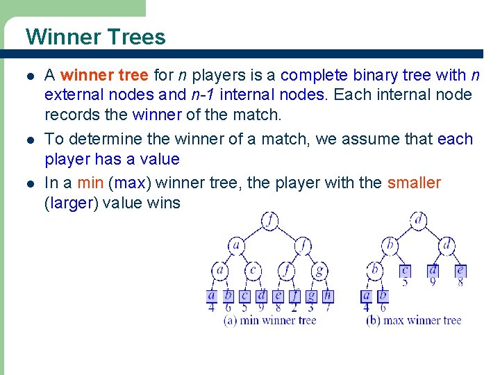
Winner Trees l l l A winner tree for n players is a complete binary tree with n external nodes and n-1 internal nodes. Each internal node records the winner of the match. To determine the winner of a match, we assume that each player has a value In a min (max) winner tree, the player with the smaller (larger) value wins

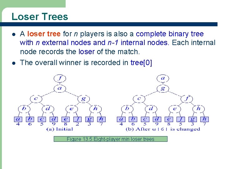
Loser Trees l l A loser tree for n players is also a complete binary tree with n external nodes and n-1 internal nodes. Each internal node records the loser of the match. The overall winner is recorded in tree[0] Figure 13. 5 Eight-player min loser trees

Bin Packing Problems

Bin Packing Problem l l l We have bins that have a capacity bin. Capacity and n objects that need to be packed into these bins Object i requires obj. Size[i], where 0 < obj. Size[i] bin. Capacity, units of capacity Feasible packing - an assignment of objects to bins so that no bin’s capacity is exceeded Optimal packing - a feasible packing that uses the fewest number of bins Goal: pack objects with the minimum number of bins The bin packing problem is an NP-hard problem

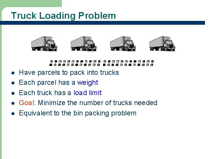
Truck Loading Problem l l l Have parcels to pack into trucks Each parcel has a weight Each truck has a load limit Goal: Minimize the number of trucks needed Equivalent to the bin packing problem

Bin Packing Approximation Algorithms l l First Fit (FF) First Fit Decreasing (FFD) Best Fit (BF) Best Fit Decreasing (BFD)

First Fit (FF) Bin Packing l l Bins are arranged in left to right order. Objects are packed one at a time in a given order. Current object is packed into the leftmost bin into which it fits. If there is no bin into which current object fits, start a new bin.

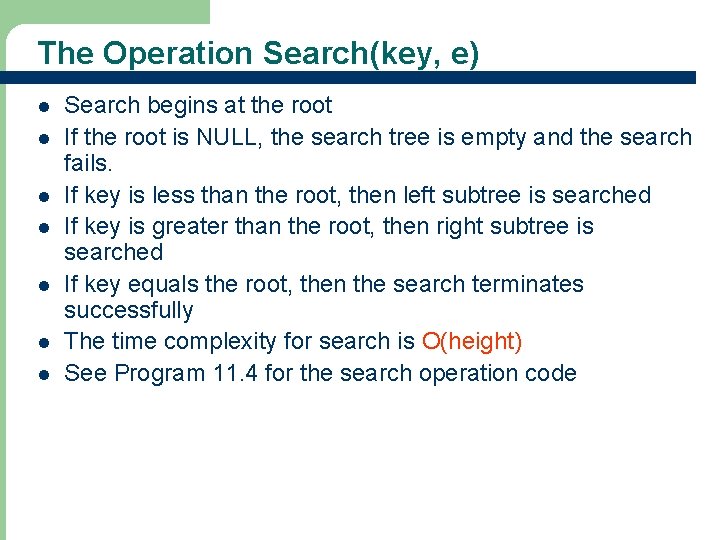
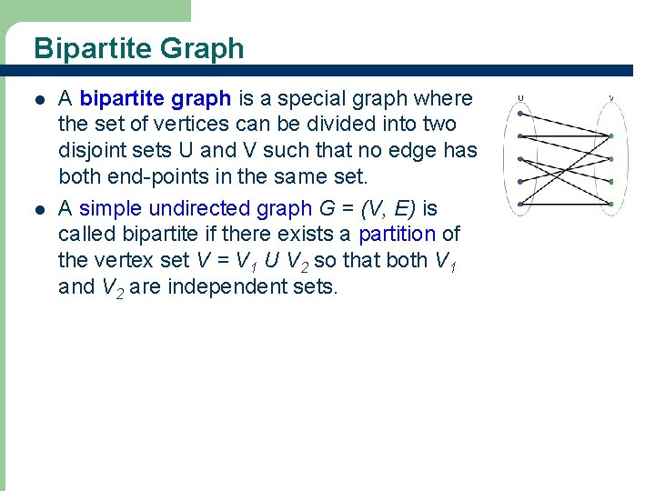
Best Fit (BF) Bin Packing l l Let bin[j]. unused. Capacity denote the capacity available in bin j Initially, the available capacity is bin. Capacity for all bins Object i is packed into the bin with the least unused. Capacity that is at least obj. Size[i] If there is no bin into which current object fits, start a new bin.

First Fit Decreasing (FFD) Bin Packing l This method is the same as FF except that the objects reordered in a decreasing size so that obj. Size[i] obj. Size[i+1], 1 i < n

Best Fit Decreasing (BFD) Bin Packing l This method is the same as BF except that the objects are reordered as for FFD

Binary Search Trees

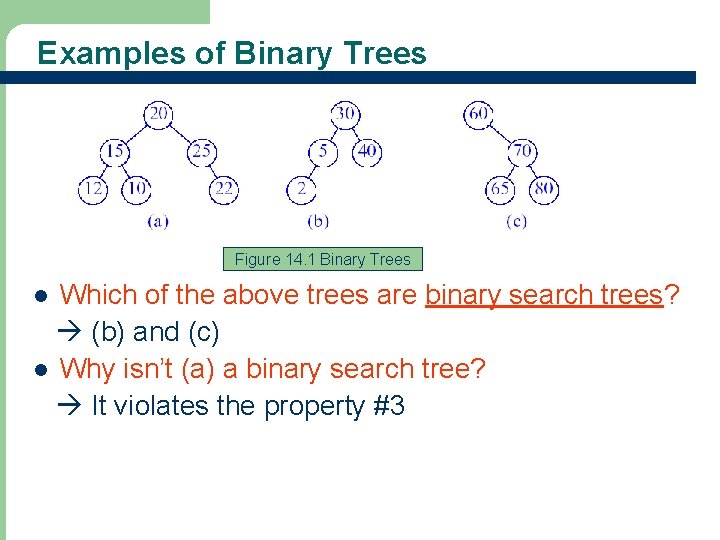
Binary Search Tree l 1. 2. 3. 4. A binary tree that may be empty. A nonempty binary search tree satisfies the following properties: Each node has a key (or value), and no two nodes have the same key (i. e. , all keys are distinct). For every node x, all keys in the left subtree of x are smaller than that in x. For every node x, all keys in the right subtree of x are larger than that in x. The left and right subtrees of the root are also binary search trees

Examples of Binary Trees Figure 14. 1 Binary Trees Which of the above trees are binary search trees? (b) and (c) l Why isn’t (a) a binary search tree? It violates the property #3 l

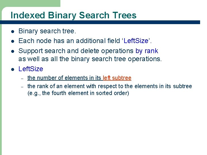
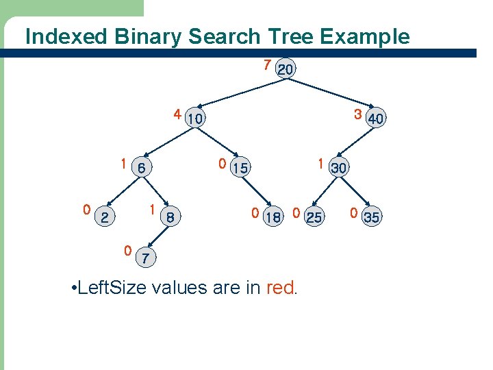
Indexed Binary Search Trees l l Binary search tree. Each node has an additional field ‘Left. Size’. Support search and delete operations by rank as well as all the binary search tree operations. Left. Size – – the number of elements in its left subtree the rank of an element with respect to the elements in its subtree (e. g. , the fourth element in sorted order)

Indexed Binary Search Tree Example 7 20 4 10 1 6 0 0 15 1 2 0 3 40 8 1 30 0 18 0 25 7 • Left. Size values are in red. 0 35

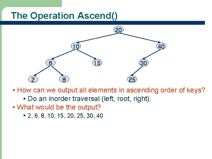
The Operation Ascend() 20 10 6 2 40 15 8 30 25 • How can we output all elements in ascending order of keys? • Do an inorder traversal (left, root, right). • What would be the output? • 2, 6, 8, 10, 15, 20, 25, 30, 40

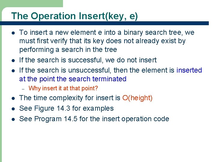
The Operation Search(key, e) l l l l Search begins at the root If the root is NULL, the search tree is empty and the search fails. If key is less than the root, then left subtree is searched If key is greater than the root, then right subtree is searched If key equals the root, then the search terminates successfully The time complexity for search is O(height) See Program 11. 4 for the search operation code

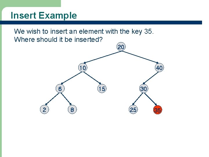
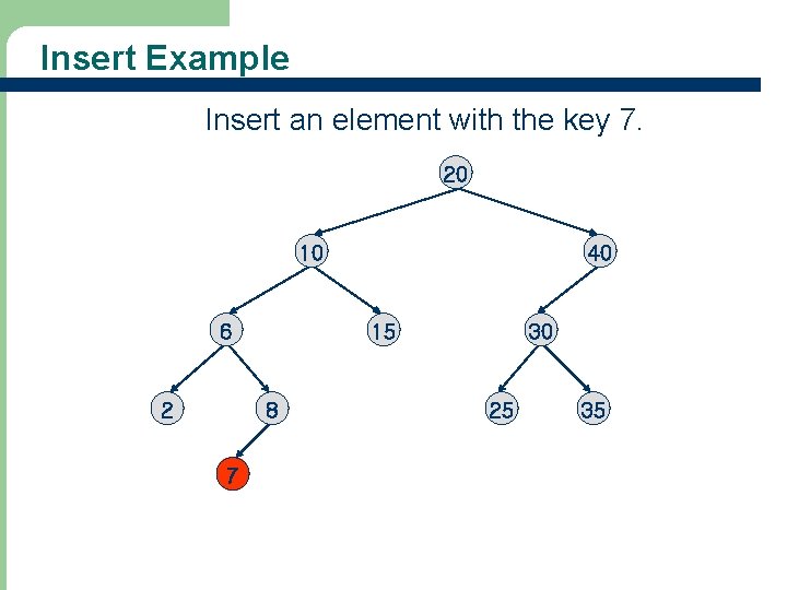
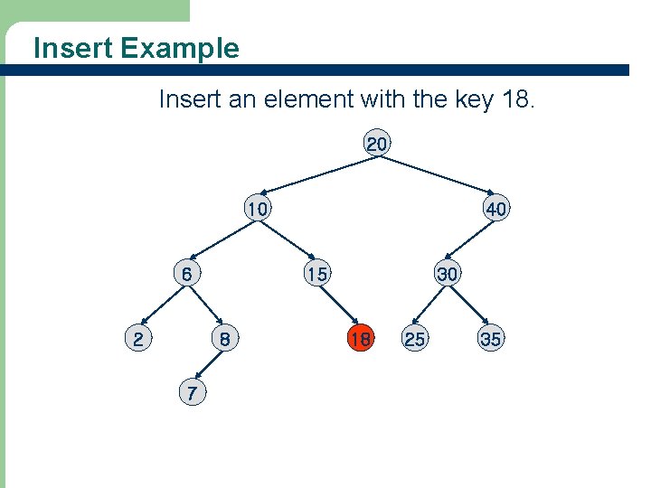
The Operation Insert(key, e) l l l To insert a new element e into a binary search tree, we must first verify that its key does not already exist by performing a search in the tree If the search is successful, we do not insert If the search is unsuccessful, then the element is inserted at the point the search terminated – l l l Why insert it at that point? The time complexity for insert is O(height) See Figure 14. 3 for examples See Program 14. 5 for the insert operation code

Insert Example We wish to insert an element with the key 35. Where should it be inserted? 20 10 6 2 40 15 8 30 25 35

Insert Example Insert an element with the key 7. 20 10 6 2 15 8 7 40 30 25 35

Insert Example Insert an element with the key 18. 20 10 6 2 15 8 7 40 30 18 25 35

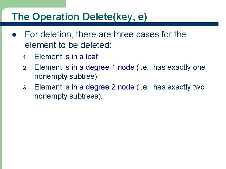
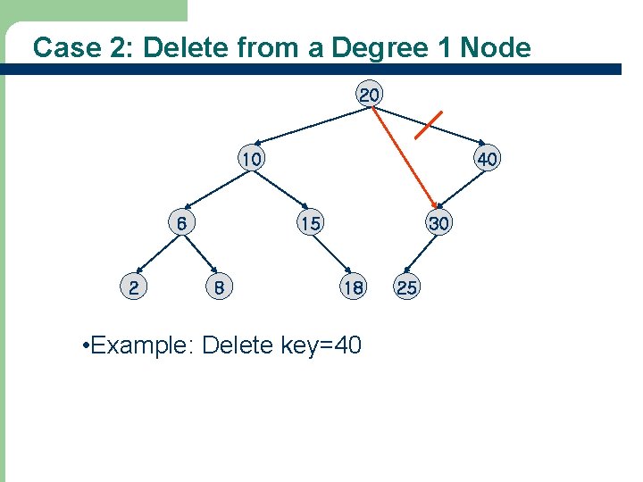
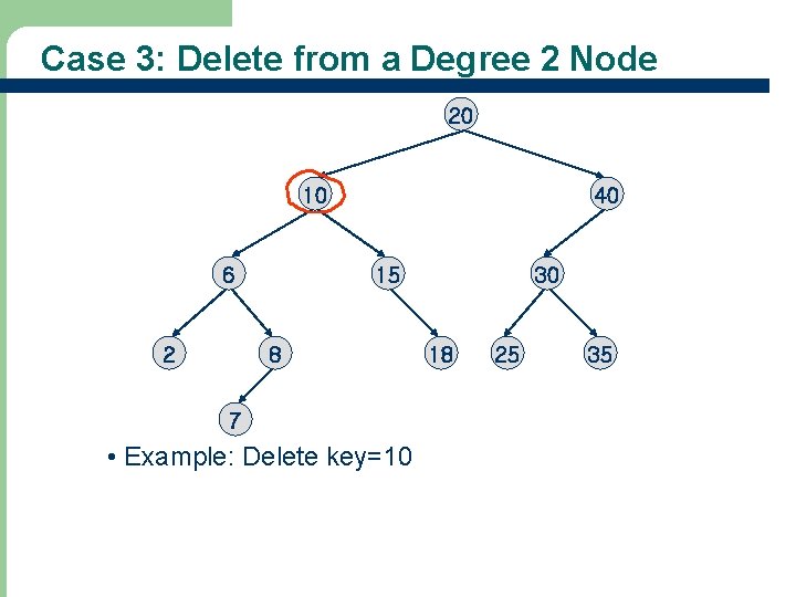
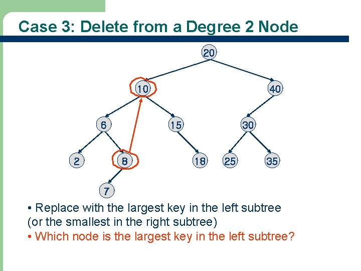
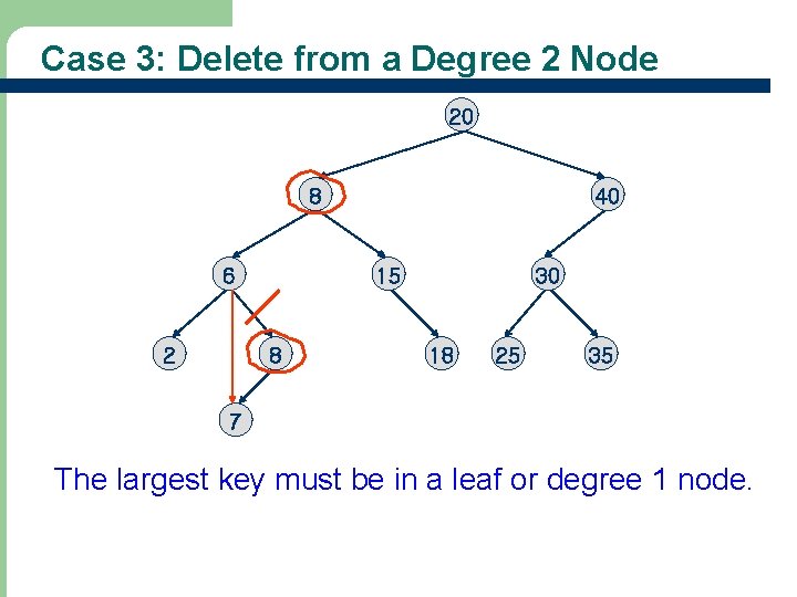
The Operation Delete(key, e) l For deletion, there are three cases for the element to be deleted: 1. 2. 3. Element is in a leaf. Element is in a degree 1 node (i. e. , has exactly one nonempty subtree). Element is in a degree 2 node (i. e. , has exactly two nonempty subtrees).

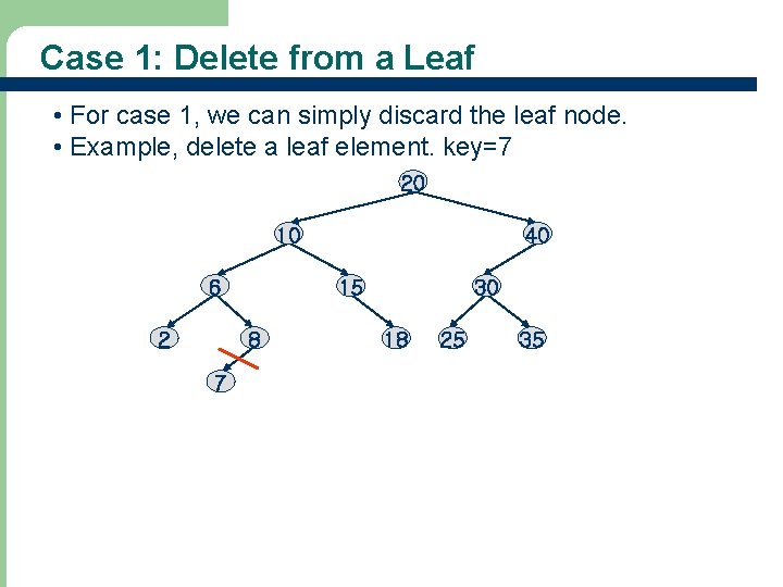
Case 1: Delete from a Leaf • For case 1, we can simply discard the leaf node. • Example, delete a leaf element. key=7 20 10 6 2 15 8 7 40 30 18 25 35

Case 2: Delete from a Degree 1 Node 20 10 6 2 40 15 8 30 18 • Example: Delete key=40 25

Case 3: Delete from a Degree 2 Node 20 10 6 2 40 15 8 7 • Example: Delete key=10 30 18 25 35

Case 3: Delete from a Degree 2 Node 20 10 6 2 40 15 8 30 18 25 35 7 • Replace with the largest key in the left subtree (or the smallest in the right subtree) • Which node is the largest key in the left subtree?

Case 3: Delete from a Degree 2 Node 20 8 6 2 40 15 8 30 18 25 35 7 The largest key must be in a leaf or degree 1 node.

AVL Trees

Balanced Binary Search Trees l l Trees with a worst-case height of O(log n) are called balanced trees An example of a balanced tree is AVL (Adelson. Velsky and Landis) tree

AVL Tree Definition l Binary tree. l If T is a nonempty binary tree with TL and TR as its left and right subtrees, then T is an AVL tree iff 1. 2. TL and TR are AVL trees, and |h. L – h. R| 1 where h. L and h. R are the heights of TL and TR, respectively

AVL Search Trees l An AVL search tree is a binary search tree that is also an AVL tree

Indexed AVL Search Trees l An indexed AVL search tree is an indexed binary search tree that is also an AVL tree

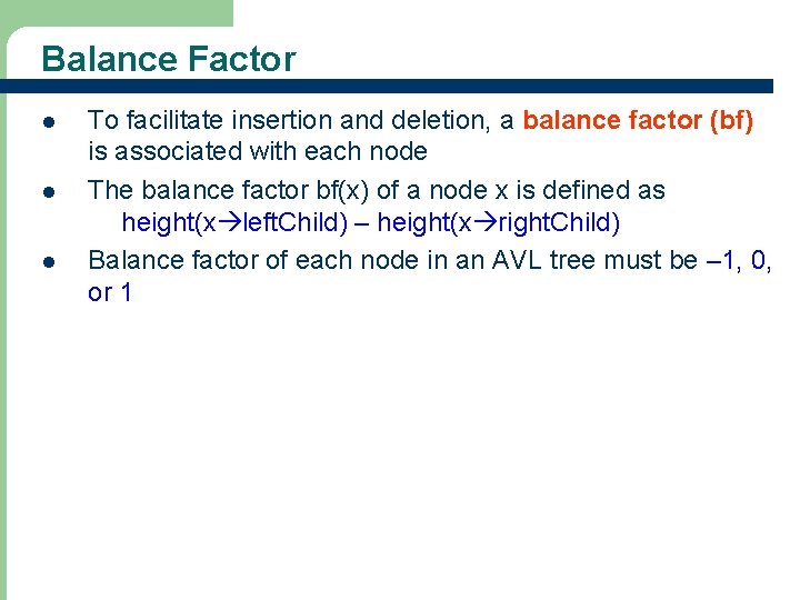
Balance Factor l l l To facilitate insertion and deletion, a balance factor (bf) is associated with each node The balance factor bf(x) of a node x is defined as height(x left. Child) – height(x right. Child) Balance factor of each node in an AVL tree must be – 1, 0, or 1

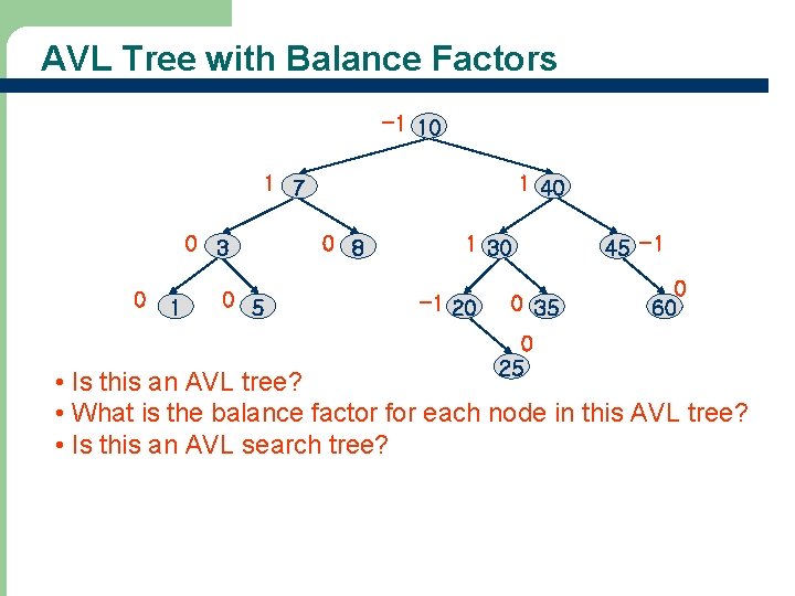
AVL Tree with Balance Factors -1 10 1 7 0 3 0 1 0 5 1 40 0 8 1 30 -1 20 0 35 0 25 45 -1 0 60 • Is this an AVL tree? • What is the balance factor for each node in this AVL tree? • Is this an AVL search tree?

Inserting into an AVL Search Trees l l l If we use the strategy of Program 14. 5 to insert an element into an AVL search tree, the result may not be an AVL tree That is, the tree may become unbalanced If the tree becomes unbalanced, we must adjust the tree to restore balance - this adjustment is called rotation

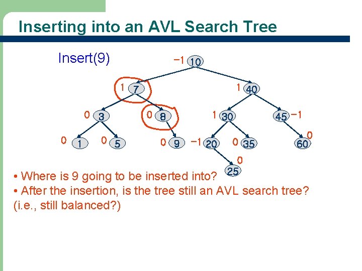
Inserting into an AVL Search Tree Insert(9) -1 10 1 7 0 3 0 1 0 5 1 40 0 8 0 9 1 30 -1 20 0 35 0 25 45 -1 0 60 • Where is 9 going to be inserted into? • After the insertion, is the tree still an AVL search tree? (i. e. , still balanced? )

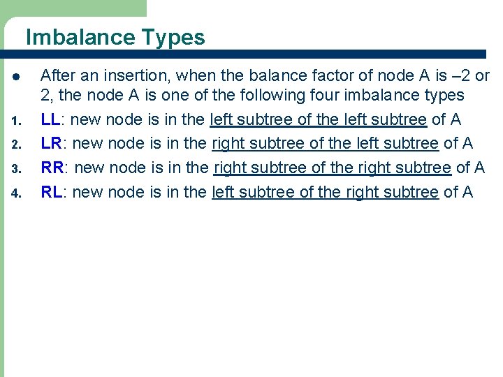
Imbalance Types l 1. 2. 3. 4. After an insertion, when the balance factor of node A is – 2 or 2, the node A is one of the following four imbalance types LL: new node is in the left subtree of A LR: new node is in the right subtree of the left subtree of A RR: new node is in the right subtree of A RL: new node is in the left subtree of the right subtree of A

Rotation Definition l To switch children and parents among two or three adjacent nodes to restore balance of a tree. l A rotation may change the depth of some nodes, but does not change their relative ordering.

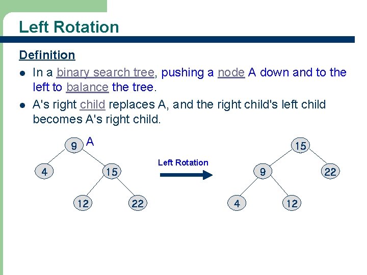
Left Rotation Definition l In a binary search tree, pushing a node A down and to the left to balance the tree. l A's right child replaces A, and the right child's left child becomes A's right child. 9 A 4 15 Left Rotation 15 12 22 9 4 22 12

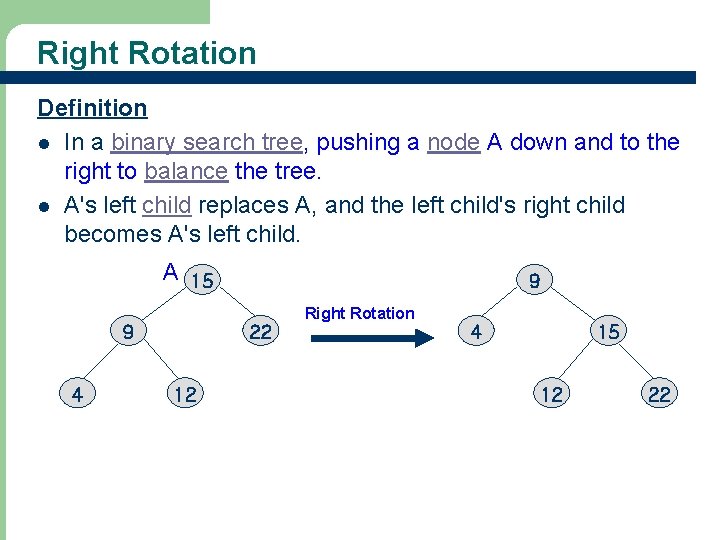
Right Rotation Definition l In a binary search tree, pushing a node A down and to the right to balance the tree. l A's left child replaces A, and the left child's right child becomes A's left child. A 15 9 4 9 22 12 Right Rotation 4 15 12 22

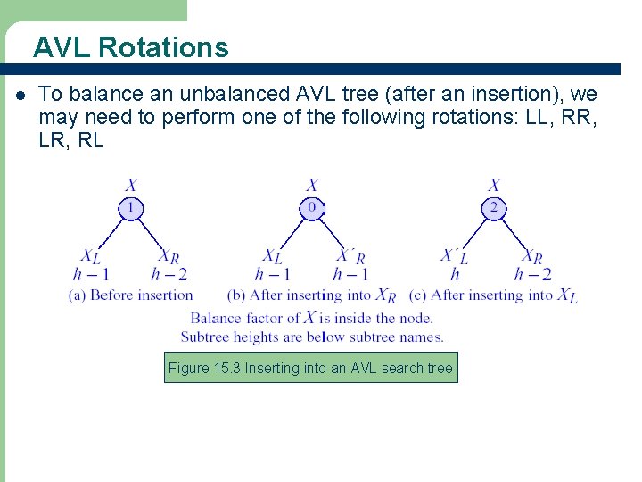
AVL Rotations l To balance an unbalanced AVL tree (after an insertion), we may need to perform one of the following rotations: LL, RR, LR, RL Figure 15. 3 Inserting into an AVL search tree

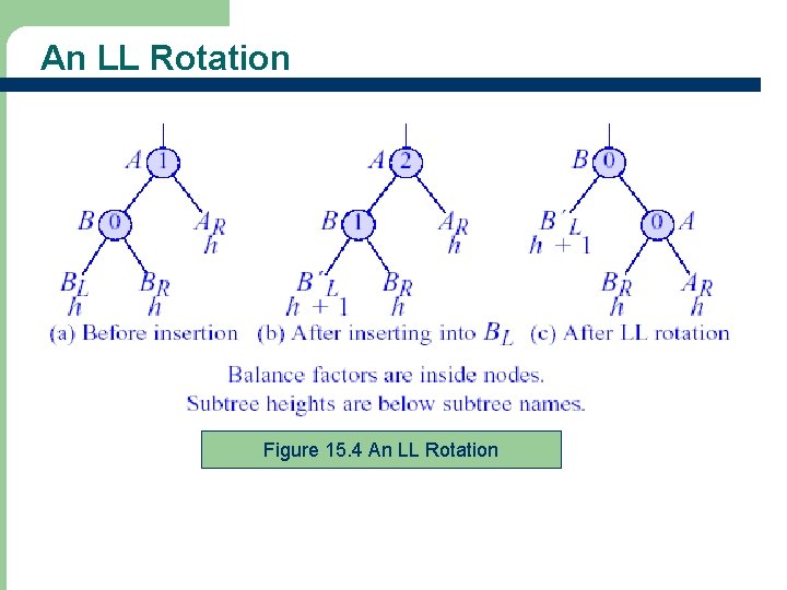
An LL Rotation Figure 15. 4 An LL Rotation

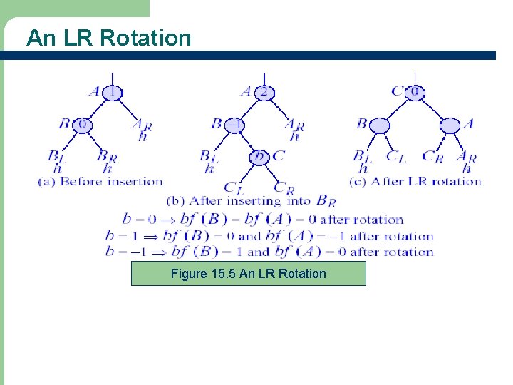
An LR Rotation Figure 15. 5 An LR Rotation

Single and Double Rotations l l l Single rotations: the transformations done to correct LL and RR imbalances Double rotations: the transformations done to correct LR and RL imbalances The transformation to correct LR imbalance can be achieved by an RR rotation followed by an LL rotation The transformation to correct RL imbalance can be achieved by an LL rotation followed by an RR rotation (do Exercise 15. 13) See Figure 15. 6 for the AVL-search-tree-insertion algorithm

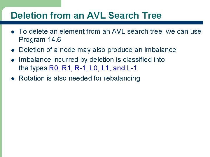
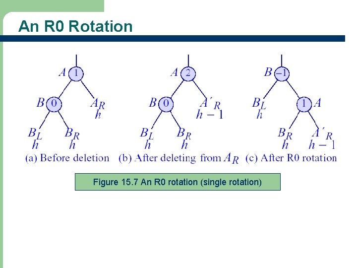
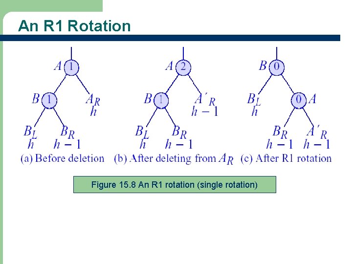
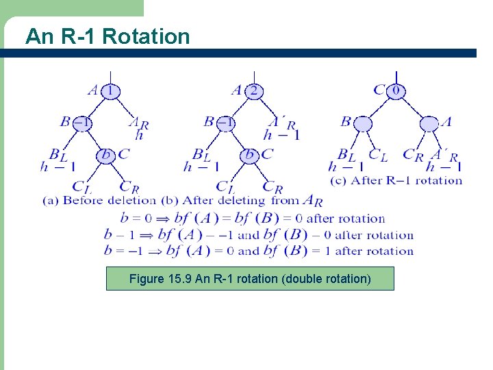
Deletion from an AVL Search Tree l l To delete an element from an AVL search tree, we can use Program 14. 6 Deletion of a node may also produce an imbalance Imbalance incurred by deletion is classified into the types R 0, R 1, R-1, L 0, L 1, and L-1 Rotation is also needed for rebalancing

An R 0 Rotation Figure 15. 7 An R 0 rotation (single rotation)

An R 1 Rotation Figure 15. 8 An R 1 rotation (single rotation)

An R-1 Rotation Figure 15. 9 An R-1 rotation (double rotation)

Graphs

Topics related to Graphs l l l Graph terminology: vertex, edge, adjacent, incident, degree, cycle, path, connected component, spanning tree Types of graphs: undirected, weighted Graph representations: adjacency matrix, array adjacency lists, linked adjacency lists Graph search methods: breath-first, depth-first search Algorithms: – – – to find a path in a graph to find the connected components of an undirected graph to find a spanning tree of a connected undirected graph

Graphs l l l l G = (V, E) V is the vertex set. Vertices are also called nodes and points. E is the edge set. Each edge connects two vertices. Edges are also called arcs and lines. Vertices i and j are adjacent vertices iff (i, j) is an edge in the graph The edge (i, j) is incident on the vertices i and j

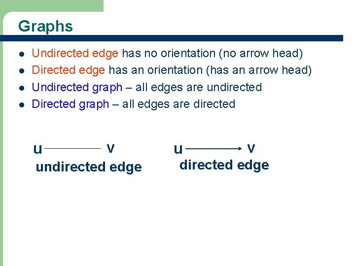
Graphs l l Undirected edge has no orientation (no arrow head) Directed edge has an orientation (has an arrow head) Undirected graph – all edges are undirected Directed graph – all edges are directed u v undirected edge u v directed edge

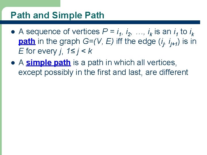
Path and Simple Path l l A sequence of vertices P = i 1, i 2, …, ik is an i 1 to ik path in the graph G=(V, E) iff the edge (ij, ij+1) is in E for every j, 1≤ j < k A simple path is a path in which all vertices, except possibly in the first and last, are different

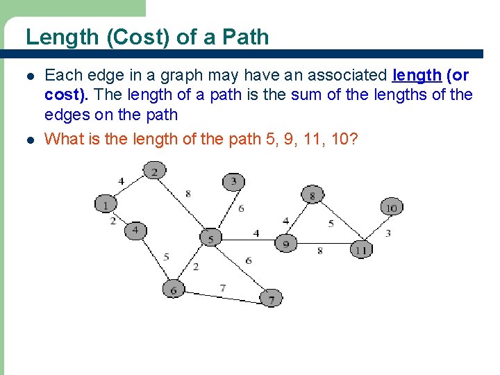
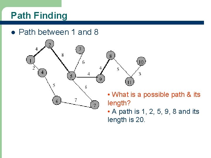
Length (Cost) of a Path l l Each edge in a graph may have an associated length (or cost). The length of a path is the sum of the lengths of the edges on the path What is the length of the path 5, 9, 11, 10?

Subgraph & Cycle l l l Let G = (V, E) be an undirected graph A graph H is a subgraph of graph G iff its vertex and edge sets are subsets of those of G A cycle is a simple path with the same start and end vertex

Spanning Tree l l l Let G = (V, E) be an undirected graph A connected undirected graph that contains no cycles is a tree A subgraph of G that contains all the vertices of G and is a tree is a spanning tree A spanning tree has n vertices and n-1 edges The spanning tree that costs the least is called the minimum-cost spanning tree

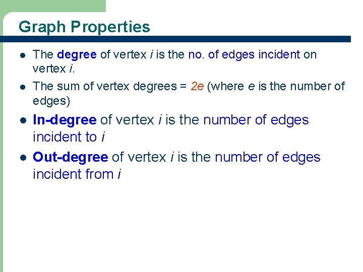
Bipartite Graph l l A bipartite graph is a special graph where the set of vertices can be divided into two disjoint sets U and V such that no edge has both end-points in the same set. A simple undirected graph G = (V, E) is called bipartite if there exists a partition of the vertex set V = V 1 U V 2 so that both V 1 and V 2 are independent sets.

Graph Properties l l The degree of vertex i is the no. of edges incident on vertex i. The sum of vertex degrees = 2 e (where e is the number of edges) In-degree of vertex i is the number of edges incident to i Out-degree of vertex i is the number of edges incident from i

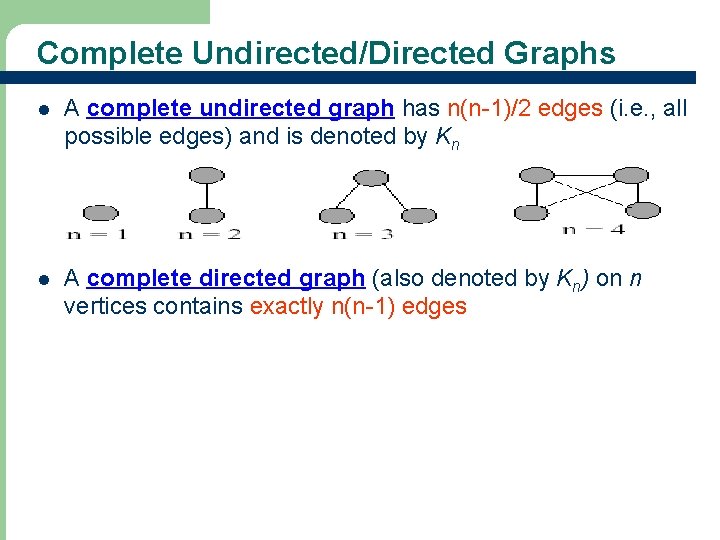
Complete Undirected/Directed Graphs l A complete undirected graph has n(n-1)/2 edges (i. e. , all possible edges) and is denoted by Kn l A complete directed graph (also denoted by Kn) on n vertices contains exactly n(n-1) edges

Path Finding l Path between 1 and 8 • What is a possible path & its length? • A path is 1, 2, 5, 9, 8 and its length is 20.

Connected Graph l l Let G = (V, E) be an undirected graph G is connected iff there is a path between every pair of vertices in G

Representation of Unweighted Graphs l The most frequently used representations for unweighted graphs are – – – Adjacency Matrix Linked adjacency lists Array adjacency lists

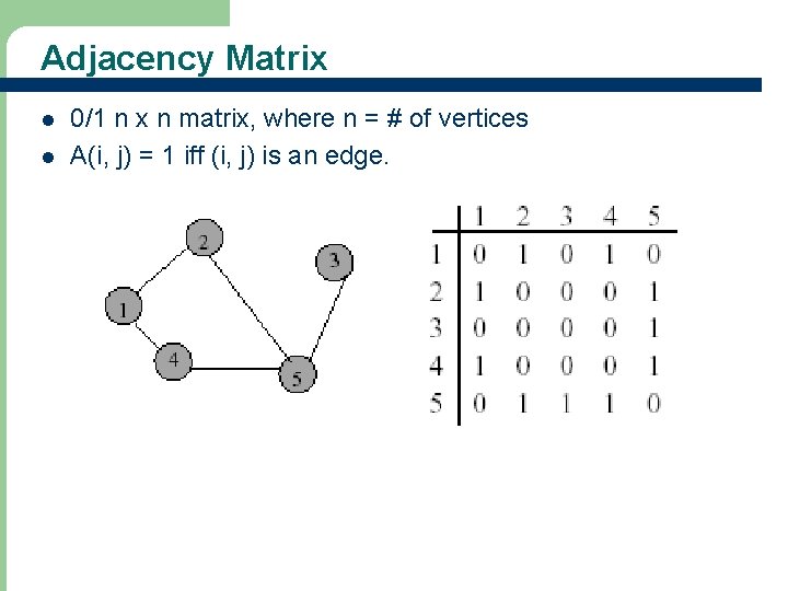
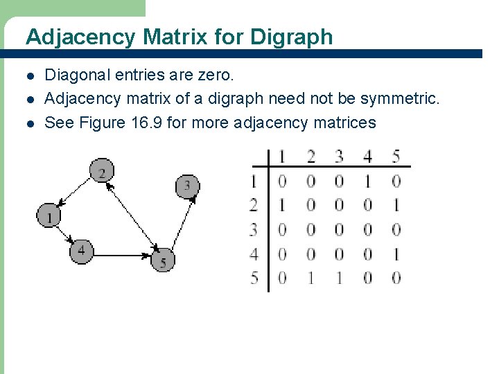
Adjacency Matrix l l 0/1 n x n matrix, where n = # of vertices A(i, j) = 1 iff (i, j) is an edge.

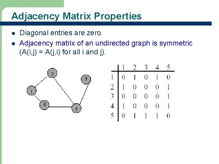
Adjacency Matrix Properties l l Diagonal entries are zero. Adjacency matrix of an undirected graph is symmetric (A(i, j) = A(j, i) for all i and j).

Adjacency Matrix for Digraph l l l Diagonal entries are zero. Adjacency matrix of a digraph need not be symmetric. See Figure 16. 9 for more adjacency matrices

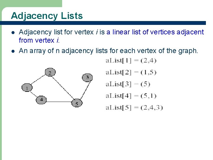
Adjacency Lists l l Adjacency list for vertex i is a linear list of vertices adjacent from vertex i. An array of n adjacency lists for each vertex of the graph.

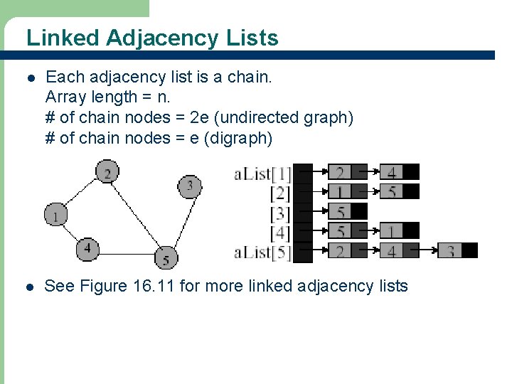
Linked Adjacency Lists l Each adjacency list is a chain. Array length = n. # of chain nodes = 2 e (undirected graph) # of chain nodes = e (digraph) l See Figure 16. 11 for more linked adjacency lists

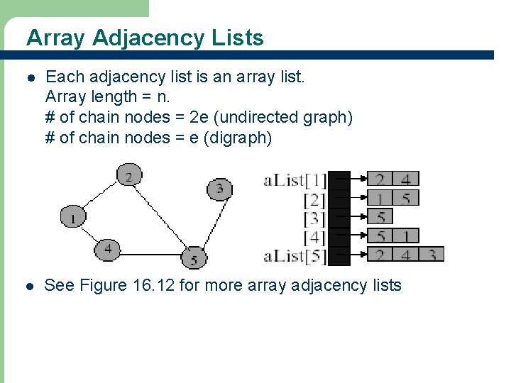
Array Adjacency Lists l Each adjacency list is an array list. Array length = n. # of chain nodes = 2 e (undirected graph) # of chain nodes = e (digraph) l See Figure 16. 12 for more array adjacency lists

Representation of Weighted Graphs l l Weighted graphs are represented with simple extensions of those used for unweighted graphs The cost-adjacency-matrix representation uses a matrix C just like the adjacency-matrix representation does Cost-adjacency matrix: C(i, j) = cost of edge (i, j) Adjacency lists: each list element is a pair (adjacent vertex, edge weight)

Graph Search Methods

Graph Search Methods l Many graph problems solved by a search method – – l Breadth-first search (BFS) – – l Finding a path from one vertex to another. Determining whether a graph is connected Find a spanning tree Finding a minimum-cost path/spanning tree Method of starting at a vertex and identifying all vertices reachable from it Similar to the level-order traversal of a binary tree Depth-first search (DFS) – – an alternative to BFS Similar to the pre-order traversal of a binary tree

Tips on the Final Exam l l l Make sure you do all the exercises mentioned in the lecture notes Make sure you understand on how to solve the problems in the assignments Good luck!

Tips on your LIFE l Have a Life Plan – – l Have a Role Model – – l Yearly life plan at the beginning of each year Plan for 5, 10, 20, 30, 40, 50 years ahead Bill Gates, Steve Jobs, Larry Page and Sergey Brin Alan Turing, Vincent Cerf and Leonard Kleinrock 안철수, 손정의, 진대제 홍원기? Have a Wonderful Life!