CSE 232 A Graduate Database Systems Arun Kumar

CSE 232 A Graduate Database Systems Arun Kumar Topic 2: Indexing and Sorting Chapters 10, 11, and 13 of Cow Book Slide ACKs: Jignesh Patel, Paris Koutris 1

Motivation for Indexing ❖ Consider the following SQL query: Movies (M) Movie. ID Name Year Director SELECT * FROM Movies WHERE Year=2017 Q: How to obtain the matching records from the file? ❖ Heap file? Need to do a linear scan! O(N) I/O and CPU ❖ “Sorted” file? Binary search! O(log 2(N)) I/O and CPU Indexing helps retrieve records faster for selective predicates! SELECT * FROM Movies WHERE Year>=2000 AND Year<2010 2

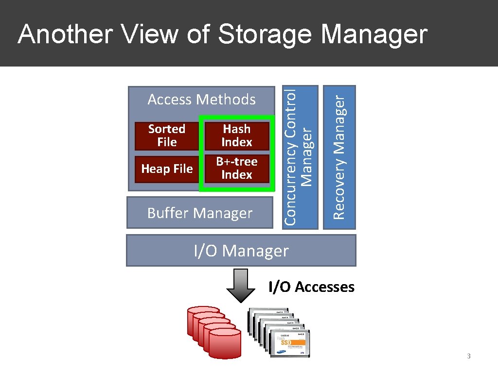
Sorted File Heap File Hash Index B+-tree Index Buffer Manager Recovery Manager Access Methods Concurrency Control Manager Another View of Storage Manager I/O Accesses 3

Indexing: Outline ❖ Overview and Terminology ❖ B+ Tree Index ❖ Hash Index ❖ Learned Index 4

Indexing ❖ Index: A data structure to speed up record retrieval ❖ Search Key: Attribute(s) on which file is indexed; also called Index Key (used interchangeably) ❖ Any permutation of any subset of a relation’s attributes can be index key for an index ❖ Index key need not be a primary/candidate key ❖ Two main types of indexes: ❖ B+ Tree index: good for both range and equality search ❖ Hash index: good for equality search 5

Overview of Indexes ❖ Need to consider efficiency of search, insert, and delete ❖ Primarily optimized to reduce (disk) I/O cost ❖ B+ Tree index: ❖ O(log. F(N)) I/O and CPU cost for equality search (N: number of “data entries”; F: “fanout” of non-leaf node) ❖ Range search, Insert, and Delete all start with an equality search ❖ Hash index: ❖ O(1) I/O and CPU cost for equality search ❖ Insert and delete start with equality search ❖ Not “good” for range search! 6

What is stored in the Index? ❖ 2 things: Search/index key values and data entries ❖ Alternatives for data entries for a given key value k: ❖ Alt. Record: Actual data records of file that match k ❖ Alt. RID: <k, RID of a record that matches k> ❖ Alt. RIDlist: <k, list of RIDs of records that match k> ❖ API for operations on records: ❖ Search (Index. Key); could be a predicate for B+Tree ❖ Insert (Index. Key, data entry) ❖ Delete (Index. Key); could be a predicate for B+Tree 7

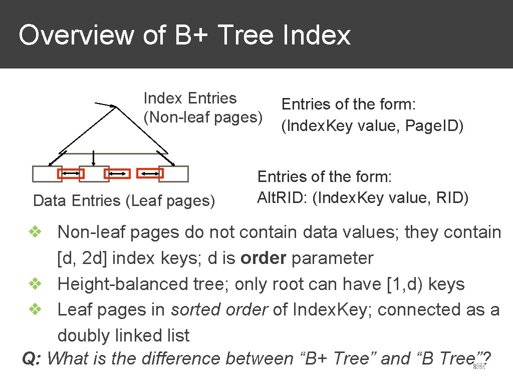
Overview of B+ Tree Index Entries (Non-leaf pages) Data Entries (Leaf pages) Entries of the form: (Index. Key value, Page. ID) Entries of the form: Alt. RID: (Index. Key value, RID) ❖ Non-leaf pages do not contain data values; they contain [d, 2 d] index keys; d is order parameter ❖ Height-balanced tree; only root can have [1, d) keys ❖ Leaf pages in sorted order of Index. Key; connected as a doubly linked list Q: What is the difference between “B+ Tree” and “B Tree”? 8

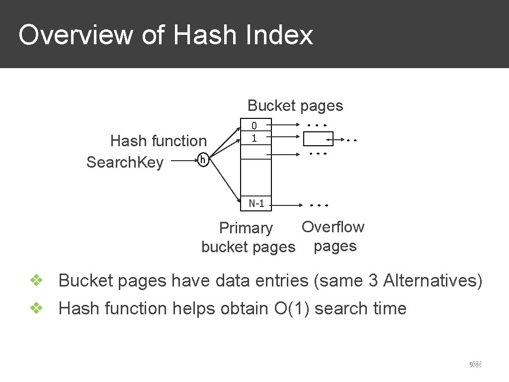
Overview of Hash Index Bucket pages Hash function h Search. Key 0 1 N-1 Overflow Primary bucket pages ❖ Bucket pages have data entries (same 3 Alternatives) ❖ Hash function helps obtain O(1) search time 9

Trade-offs of Data Entry Alternatives ❖ Pros and cons of alternatives for data entries: ❖ Alt. Record: Entire file is stored as an index! If records are long, data entries of index are large and search time could be high ❖ Alt. RID and Alt. RIDlist: Data entries typically smaller than records; often faster for equality search ❖ Alt. RIDlist has more compact data entries than Alt. RID but entries are variable-length Q: A file can have at most one Alt. Record index. Why? 10

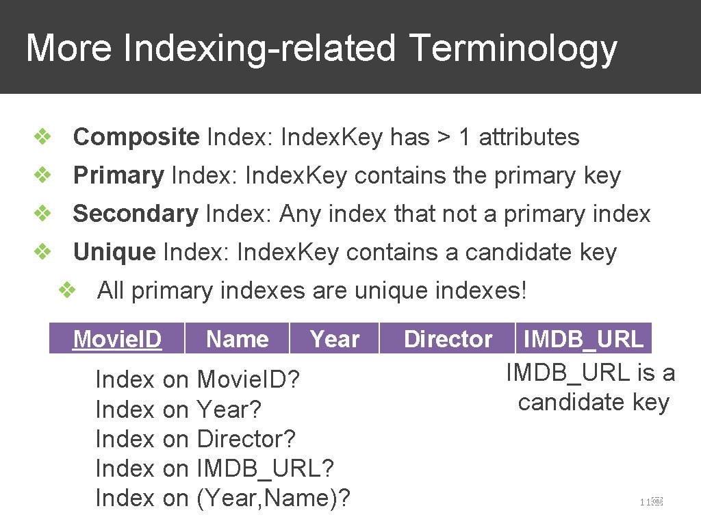
More Indexing-related Terminology ❖ Composite Index: Index. Key has > 1 attributes ❖ Primary Index: Index. Key contains the primary key ❖ Secondary Index: Any index that not a primary index ❖ Unique Index: Index. Key contains a candidate key ❖ All primary indexes are unique indexes! Movie. ID Name Year Index on Movie. ID? Index on Year? Index on Director? Index on IMDB_URL? Index on (Year, Name)? Director IMDB_URL is a candidate key 11

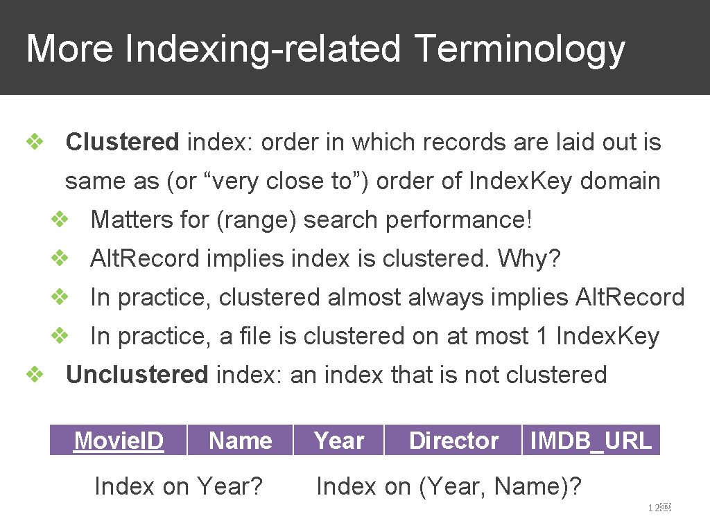
More Indexing-related Terminology ❖ Clustered index: order in which records are laid out is same as (or “very close to”) order of Index. Key domain ❖ Matters for (range) search performance! ❖ Alt. Record implies index is clustered. Why? ❖ In practice, clustered almost always implies Alt. Record ❖ In practice, a file is clustered on at most 1 Index. Key ❖ Unclustered index: an index that is not clustered Movie. ID Name Index on Year? Year Director IMDB_URL Index on (Year, Name)? 12

Indexing: Outline ❖ Overview and Terminology ❖ B+ Tree Index ❖ Hash Index ❖ Learned Index 13

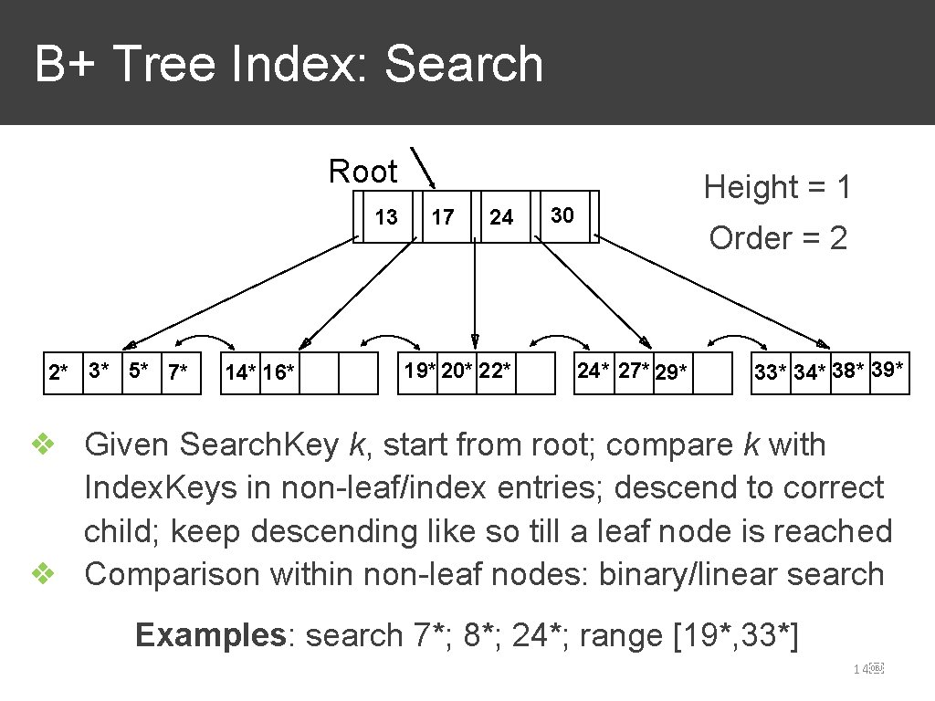
B+ Tree Index: Search Root 13 2* 3* 5* 7* 14* 16* 17 24 19* 20* 22* Height = 1 30 Order = 2 24* 27* 29* 33* 34* 38* 39* ❖ Given Search. Key k, start from root; compare k with Index. Keys in non-leaf/index entries; descend to correct child; keep descending like so till a leaf node is reached ❖ Comparison within non-leaf nodes: binary/linear search Examples: search 7*; 8*; 24*; range [19*, 33*] 14

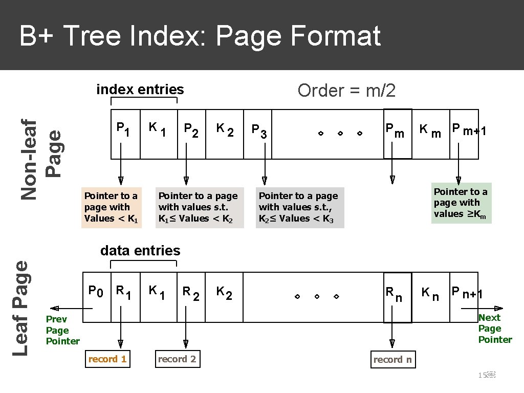
B+ Tree Index: Page Format Order = m/2 Non-leaf Page index entries P 1 Pointer to a page with Values < K 1 P 2 K 2 Pointer to a page with values s. t. K 1≤ Values < K 2 P 3 Pm K m P m+1 Pointer to a page with values ≥Km Pointer to a page with values s. t. , K 2≤ Values < K 3 Leaf Page data entries P 0 R 1 K 1 R 2 K 2 Rn K n P n+1 Next Page Pointer Prev Page Pointer record 1 record 2 record n 15

B+ Trees in Practice ❖ Typical order value: 100 (so, non-leaf node can have up to 200 index keys) ❖ Typical occupancy: 67%; so, typical “fanout” = 133 ❖ Computing the tree’s capacity using fanout: ❖ Height 1 stores 133 leaf pages ❖ Height 4 store 1334 = 312, 900, 700 leaf pages ❖ Typically, higher levels of B+Tree cached in buffer pool ❖ Level 0 (root) = 1 page = 8 KB ❖ Level 1 = 133 pages ~ 1 MB ❖ Level 2 = 17, 689 pages ~ 138 MB and so on 16

B+ Tree Index: Insert ❖ Search for correct leaf L ❖ Insert data entry into L; if L has enough space, done! Otherwise, must split L (into new L and a new leaf L’) ❖ Redistribute entries evenly, copy up middle key ❖ Insert index entry pointing to L’ into parent of L ❖ A split might have to propagate upwards recursively: ❖ To split non-leaf node, redistribute entries evenly, but push up the middle key (not copy up, as in leaf splits!) ❖ Splits “grow” the tree; root split increases height. ❖ Tree growth: gets wider or one level taller at top. 17

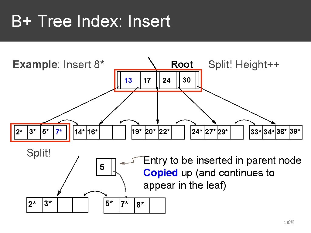
B+ Tree Index: Insert Example: Insert 8* Root 13 2* 3* 5* 7* 30 24* 27* 29* 33* 34* 38* 39* Entry to be inserted in parent node Copied up (and continues to appear in the leaf) 5 3* 24 19* 20* 22* 14* 16* Split! 2* 17 Split! Height++ 5* 7* 8* 18

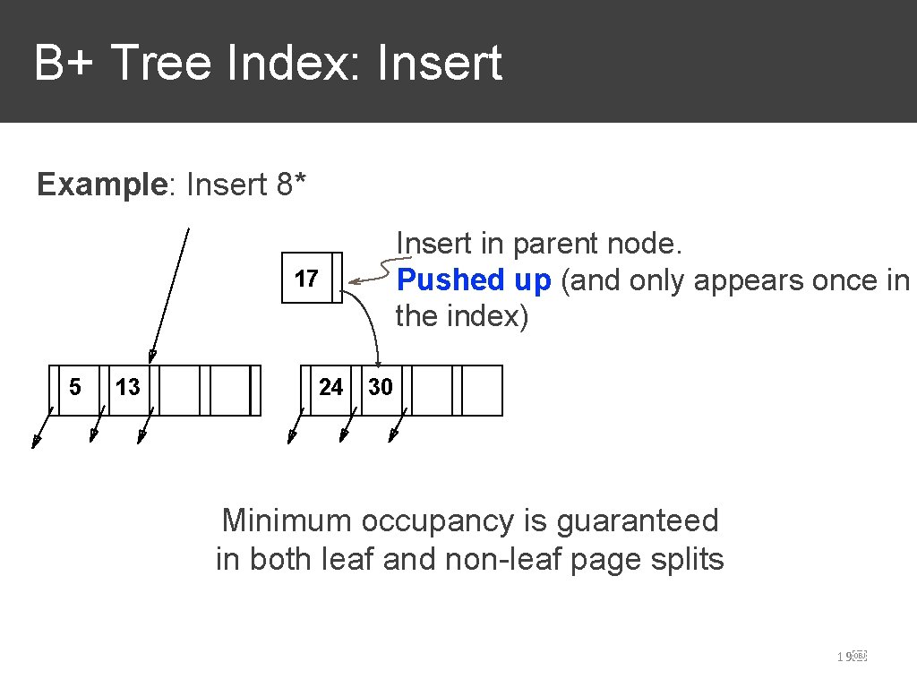
B+ Tree Index: Insert Example: Insert 8* 17 5 13 Insert in parent node. Pushed up (and only appears once in the index) 24 30 Minimum occupancy is guaranteed in both leaf and non-leaf page splits 19

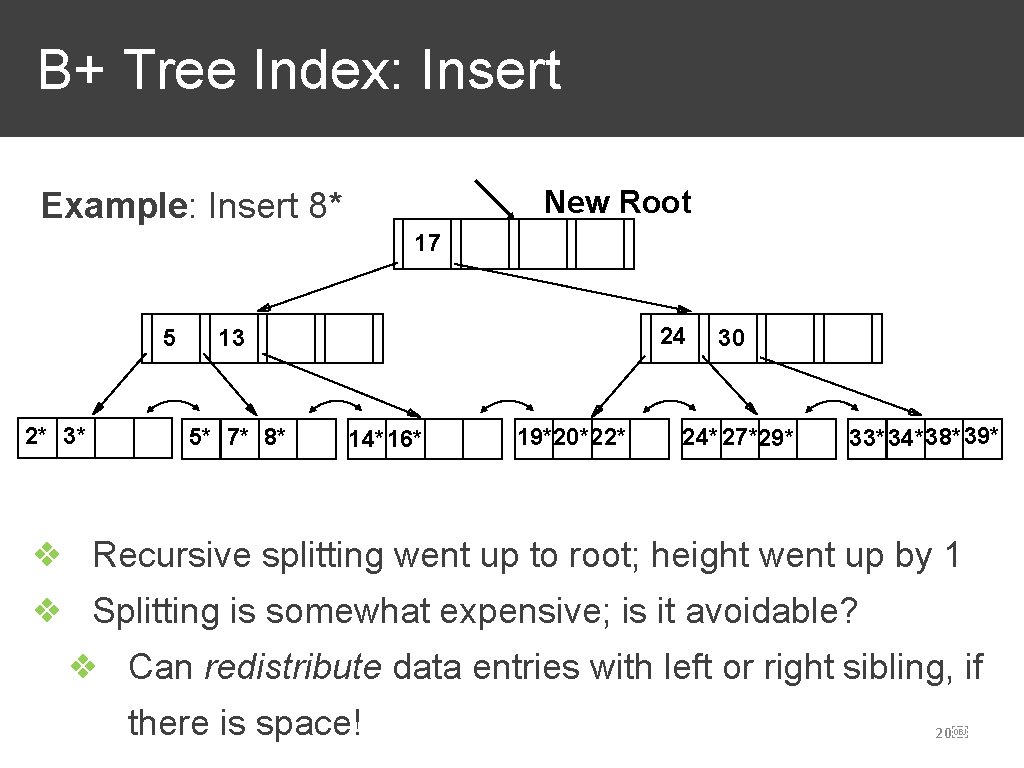
B+ Tree Index: Insert New Root Example: Insert 8* 17 5 2* 3* 24 13 5* 7* 8* 14*16* 19*20*22* 30 24* 27*29* 33*34* 38* 39* ❖ Recursive splitting went up to root; height went up by 1 ❖ Splitting is somewhat expensive; is it avoidable? ❖ Can redistribute data entries with left or right sibling, if there is space! 20

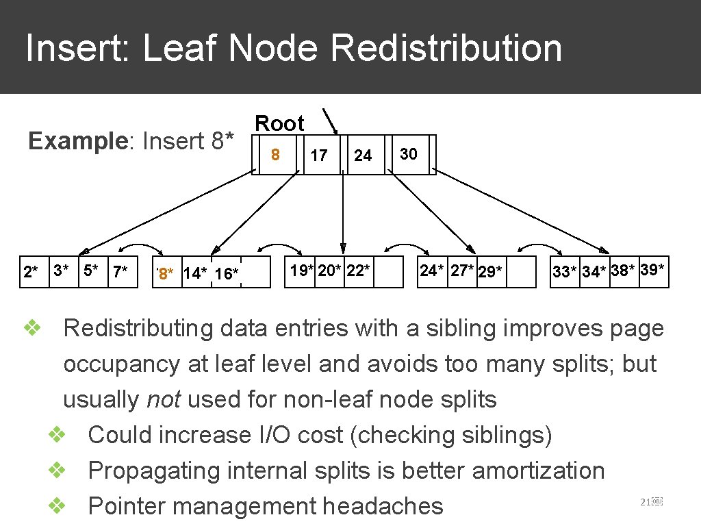
Insert: Leaf Node Redistribution Example: Insert 8* 2* 3* 5* 7* 14* 16* 8* 14* Root 8 13 17 24 19* 20* 22* 30 24* 27* 29* 33* 34* 38* 39* ❖ Redistributing data entries with a sibling improves page occupancy at leaf level and avoids too many splits; but usually not used for non-leaf node splits ❖ Could increase I/O cost (checking siblings) ❖ Propagating internal splits is better amortization 21 ❖ Pointer management headaches

B+ Tree Index: Delete ❖ Start at root, find leaf L where entry belongs ❖ Remove the entry; if L is at least half-full, done! Else, if L has only d-1 entries: ❖ Try to re-distribute, borrowing from sibling L’ ❖ If re-distribution fails, merge L and L’ into single leaf ❖ If merge occurred, must delete entry (pointing to L or sibling) from parent of L. ❖ A merge might have to propagate upwards recursively to root, which decreases height by 1 22

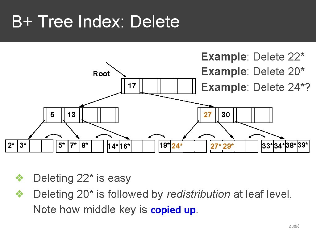
B+ Tree Index: Delete Example: Delete 22* Example: Delete 20* Example: Delete 24*? Root 17 5 2* 3* 24 27 13 5* 7* 8* 14*16* 19* 20* 24* 22* 30 24* 27* 29*29* 33*34* 38* 39* ❖ Deleting 22* is easy ❖ Deleting 20* is followed by redistribution at leaf level. Note how middle key is copied up. 23

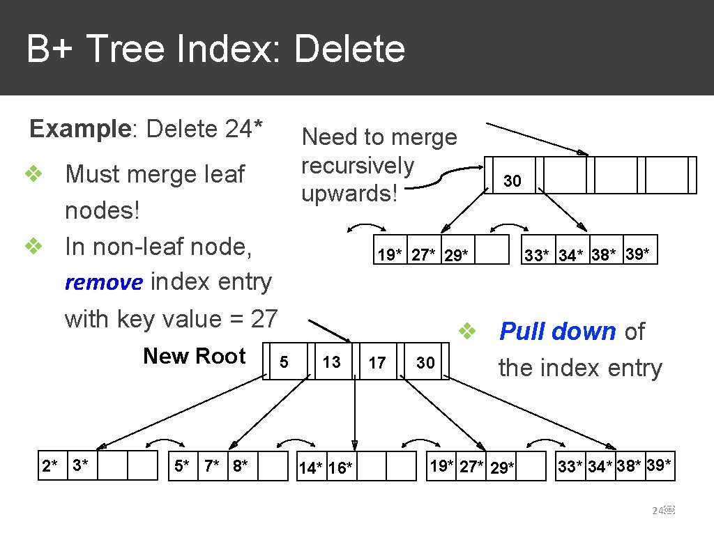
B+ Tree Index: Delete Example: Delete 24* Need to merge recursively upwards! ❖ Must merge leaf nodes! ❖ In non-leaf node, remove index entry with key value = 27 New Root 2* 3* 5* 7* 8* 30 19* 27* 29* 5 13 14* 16* 17 30 33* 34* 38* 39* ❖ Pull down of the index entry 19* 27* 29* 33* 34* 38* 39* 24

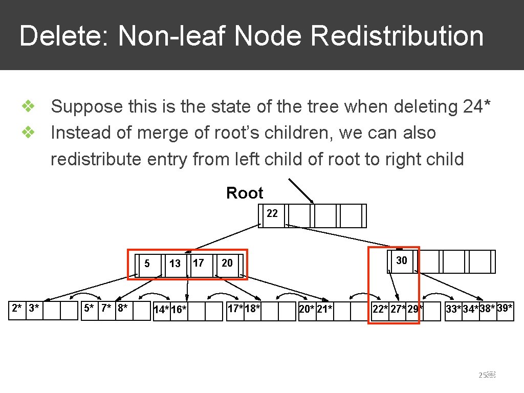
Delete: Non-leaf Node Redistribution ❖ Suppose this is the state of the tree when deleting 24* ❖ Instead of merge of root’s children, we can also redistribute entry from left child of root to right child Root 22 5 2* 3* 5* 7* 8* 13 14* 16* 17 30 20 17* 18* 20* 21* 22* 27* 29* 33* 34* 38* 39* 25

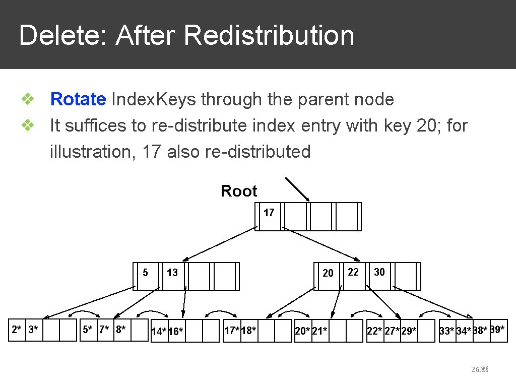
Delete: After Redistribution ❖ Rotate Index. Keys through the parent node ❖ It suffices to re-distribute index entry with key 20; for illustration, 17 also re-distributed Root 17 5 2* 3* 5* 7* 8* 13 14* 16* 20 17* 18* 20* 21* 22 30 22* 27* 29* 33* 34* 38* 39* 26

Delete: Redistribution Preferred ❖ Unlike Insert, where redistribution is discouraged for nonleaf nodes, Delete prefers redistribution over merge decisions at both leaf or non-leaf levels. Why? ❖ Files usually grow, not shrink; deletions are rare! ❖ High chance of redistribution success (high fanouts) ❖ Only need to propagate changes to parent node 27

Handling Duplicates/Repetitions ❖ Many data entries could have same Index. Key value ❖ Related to Alt. RIDlist vs Alt. RID for data entries ❖ Also, single data entry could still span multiple pages ❖ Solution 1: ❖ All data entries with a given Index. Key value reside on a single page ❖ Use “overflow” pages, if needed (not inside leaf list) ❖ Solution 2: ❖ Allow repeated Index. Key values among data entries ❖ Modify Search appropriately ❖ Use RID to get a unique composite key! 28

Order Concept in Practice ❖ In practice, order (d) concept replaced by physical space criterion: at least half-full ❖ Non-leaf pages can typically hold many more entries than leaf pages, since leaf pages could have long data records (Alt. Record) or RID lists (Alt. RIDlist) ❖ Often, different nodes could have different # entries: ❖ Variable sized Index. Key ❖ Alt. Record and variable-sized data records ❖ Alt. RIDlist could leads to different numbers of data entries sharing an Index. Key value 29

B+ Tree Index: Bulk Loading ❖ Given an existing file we want to index, multiple recordat-a-time Inserts are wasteful (too many Index. Keys!) ❖ Bulk loading avoids this overhead; reduces I/O cost ❖ 1) Sort data entries by Index. Key (Alt. Record sorts file!) ❖ 2) Create empty root page; copy leftmost Index. Key of leftmost leaf page to root (non-leaf) and assign child ❖ 3) Go left to right; Insert only leftmost Index. Key from each leaf page into index as usual (NB: fewer keys!) ❖ 4) When non-leaf fills up, follow usual Split procedure and recurse upwards, if needed 30

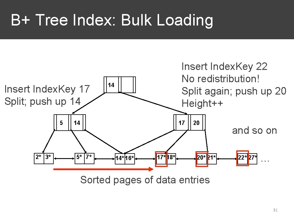
B+ Tree Index: Bulk Loading Insert Index. Key 17 Split; push up 14 5 2* 3* Insert Index. Key 22 No redistribution! Split again; push up 20 Height++ 14 14 5* 7* 17 14* 16* 17* 18* 20 20* 21* and so on 22* 27* … Sorted pages of data entries 31

Indexing: Outline ❖ Overview and Terminology ❖ B+ Tree Index ❖ Hash Index ❖ Learned Index 32

Overview of Hash Indexing ❖ Reduces search cost to nearly O(1) ❖ Good for equality search (but not for range search) ❖ Many variants: ❖ Static hashing ❖ Extendible hashing ❖ Linear hashing, etc. (we will not discuss these) 33

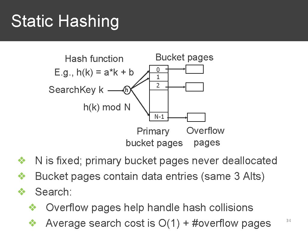
Static Hashing Hash function E. g. , h(k) = a*k + b Search. Key k h Bucket pages 0 1 2 h(k) mod N N-1 Overflow Primary bucket pages ❖ N is fixed; primary bucket pages never deallocated ❖ Bucket pages contain data entries (same 3 Alts) ❖ Search: ❖ Overflow pages help handle hash collisions ❖ Average search cost is O(1) + #overflow pages 34

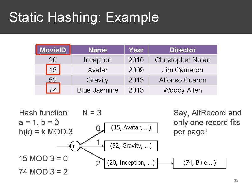
Static Hashing: Example Movie. ID 20 15 52 74 Name Inception Avatar Gravity Blue Jasmine Hash function: a = 1, b = 0 h(k) = k MOD 3 h 15 MOD 3 = 0 74 MOD 3 = 2 Year 2010 2009 2013 N=3 0 (15, Avatar, …) 1 (52, Gravity, …) 2 (20, Inception, …) Director Christopher Nolan Jim Cameron Alfonso Cuaron Woody Allen Say, Alt. Record and only one record fits per page! (74, Blue …) 35

Static Hashing: Insert and Delete ❖ Insert: ❖ Equality search; find space on primary bucket page ❖ If not enough space, add overflow page ❖ Delete: ❖ Equality search; delete record ❖ If overflow page becomes empty, remove it ❖ Primary bucket pages are never removed! 36

Static Hashing: Issues ❖ Since N is fixed, #overflow pages might grow and degrade search cost; deletes waste a lot of space ❖ Full reorg. is expensive and could block query proc. ❖ Skew in hashing: ❖ Could be due to “bad” hash function that does not “spread” values—but this issue is well-studied/solved ❖ Could be due to skew in the data (duplicates); this could cause more overflow pages—difficult to resolve Extendible (dynamic) hashing helps resolve first two issues 37

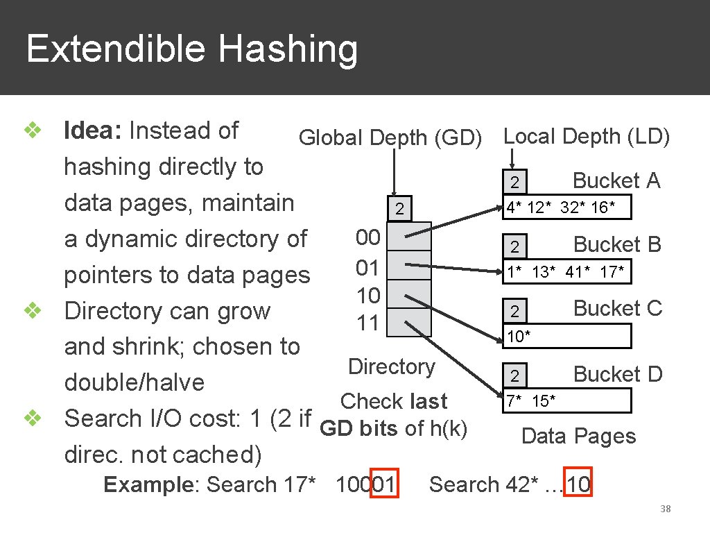
Extendible Hashing ❖ Idea: Instead of Global Depth (GD) Local Depth (LD) hashing directly to 2 Bucket A data pages, maintain 4* 12* 32* 16* 2 00 a dynamic directory of Bucket B 2 01 1* 13* 41* 17* pointers to data pages 10 Bucket C 2 ❖ Directory can grow 11 10* and shrink; chosen to Directory Bucket D 2 double/halve 7* 15* Check last ❖ Search I/O cost: 1 (2 if GD bits of h(k) Data Pages direc. not cached) Example: Search 17* 10001 Search 42* … 10 38

Extendible Hashing: Insert ❖ Search for k; if data page has space, add record; done ❖ If data page has no more space: ❖ If LD < GD, create Split Image of bucket; LD++ for both bucket and split image; insert record properly ❖ If LD == GD, create Split Image; LD++ for both buckets; insert record; but also, double the directory and GD++! Duplicate other direc. pointers properly ❖ Direc. typically grows in spurts 39

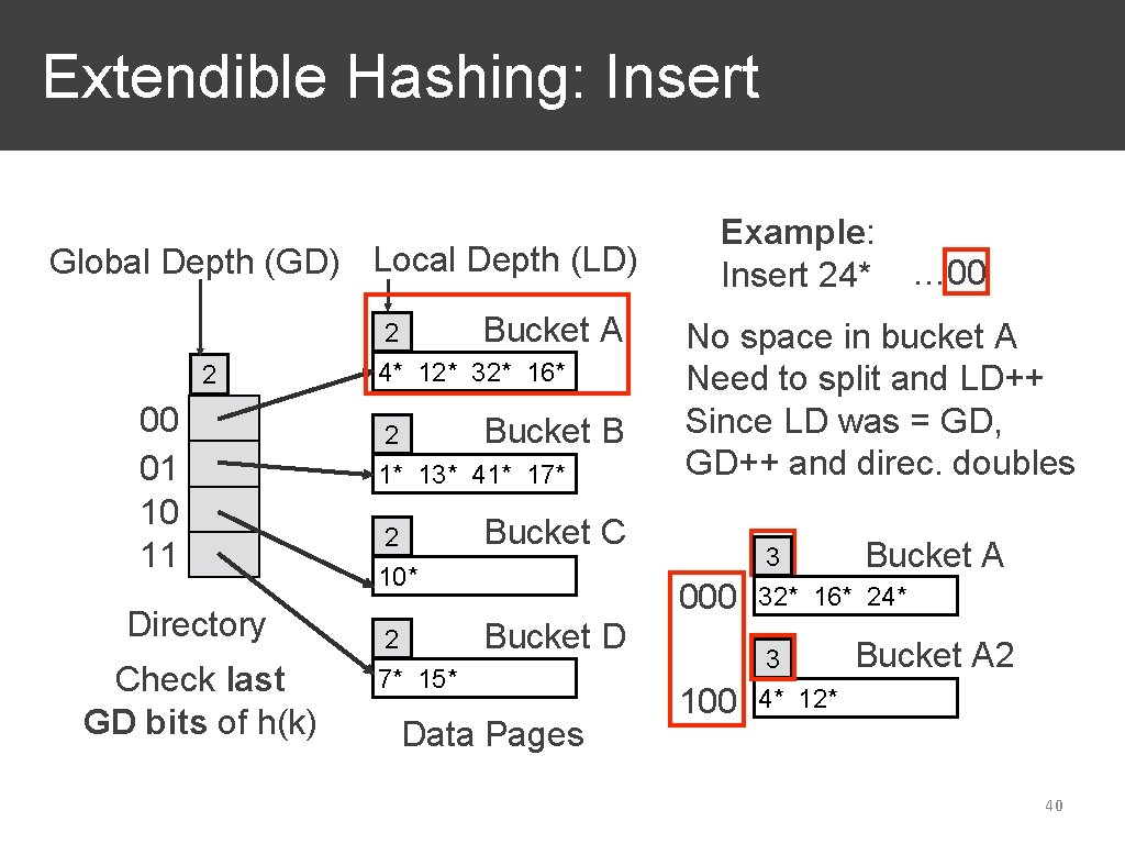
Extendible Hashing: Insert Global Depth (GD) Local Depth (LD) 2 00 01 10 11 Directory Check last GD bits of h(k) 2 Bucket 4* 12* 32* 16* A Bucket 2 1* 13* 41* 17* B 2 10* Bucket C 2 7* 15* Bucket D Data Pages Example: Insert 24* … 00 No space in bucket A Need to split and LD++ Since LD was = GD, GD++ and direc. doubles 000 3 Bucket 32* 16* 24* 100 3 4* 12* A Bucket A 2 40

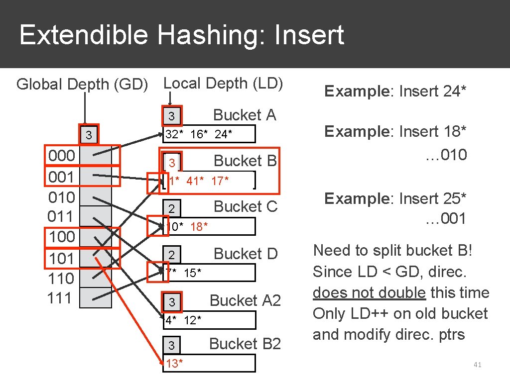
Extendible Hashing: Insert Global Depth (GD) Local Depth (LD) 3 000 001 010 011 100 101 110 111 3 Bucket 32* 16* 24* A Bucket 2 3 1* 1* 13* 41* 17* B 2 10* 18* Bucket C 2 7* 15* Bucket D 3 4* 12* Bucket A 2 3 13* Bucket B 2 Example: Insert 24* Example: Insert 18* … 010 Example: Insert 25* … 001 Need to split bucket B! Since LD < GD, direc. does not double this time Only LD++ on old bucket and modify direc. ptrs 41

Extendible Hashing: Delete ❖ Search for k; delete record on data page ❖ If data page becomes empty, we can merge with another data page with same last GD-1 bits (its “historical split image”) and do LD--; update direc. ptrs ❖ If all splits images get merged back and all buckets have LD = GD-1, shrink direc. by half; GD-NB: Never does a bucket’s LD become > GD! 42

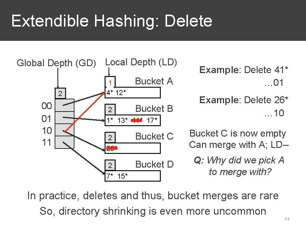
Extendible Hashing: Delete Global Depth (GD) Local Depth (LD) 2 00 01 10 11 2 1 4* 12* Bucket A Example: Delete 41* … 01 B Example: Delete 26* … 10 2 26* Bucket C is now empty Can merge with A; LD-- 2 7* 15* Bucket D Q: Why did we pick A to merge with? Bucket 2 1* 13* 41* 17* In practice, deletes and thus, bucket merges are rare So, directory shrinking is even more uncommon 43

Static Hashing vs Extendible Hashing Q: Why not let N in static hashing grow and shrink too? ❖ Extendible hash direc. size is typically much smaller than data pages; with static hash, reorg. of all data pages is far more expensive ❖ Hashing skew is a common issue for both; in static hash, this could lead to large # overflow pages; in extendible hash, this could blow up direc. size (this is OK) ❖ If too many data entries share search key (duplicates), overflow pages needed for extendible hash too! 44

Indexing: Outline ❖ Overview and Terminology ❖ B+ Tree Index ❖ Hash Index ❖ Learned Index 45

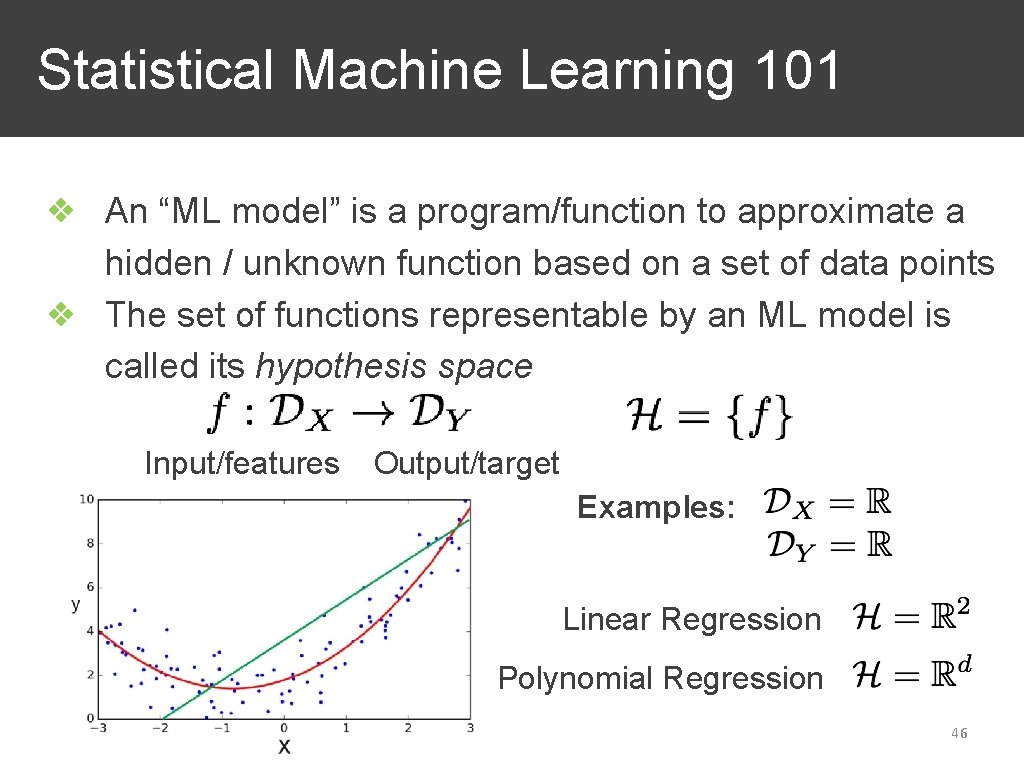
Statistical Machine Learning 101 ❖ An “ML model” is a program/function to approximate a hidden / unknown function based on a set of data points ❖ The set of functions representable by an ML model is called its hypothesis space Input/features Output/target Examples: Linear Regression Polynomial Regression 46

Statistical Machine Learning 101 ❖ Most ML models are parametric; an ML model’s learning algorithm is a program to help pick a specific function from its hypothesis space, i. e. , set parameter values ❖ Accuracy of ML model quantified by how well the picked function “fits” the observed data ❖ Two kinds of accuracy: “train” vs “test” ❖ Train is on same data seen by learning algorithm ❖ Test is on held out data; evaluates “generalization” ❖ Different ML models represent different sets of functions and thus, typically yield different accuracy 47

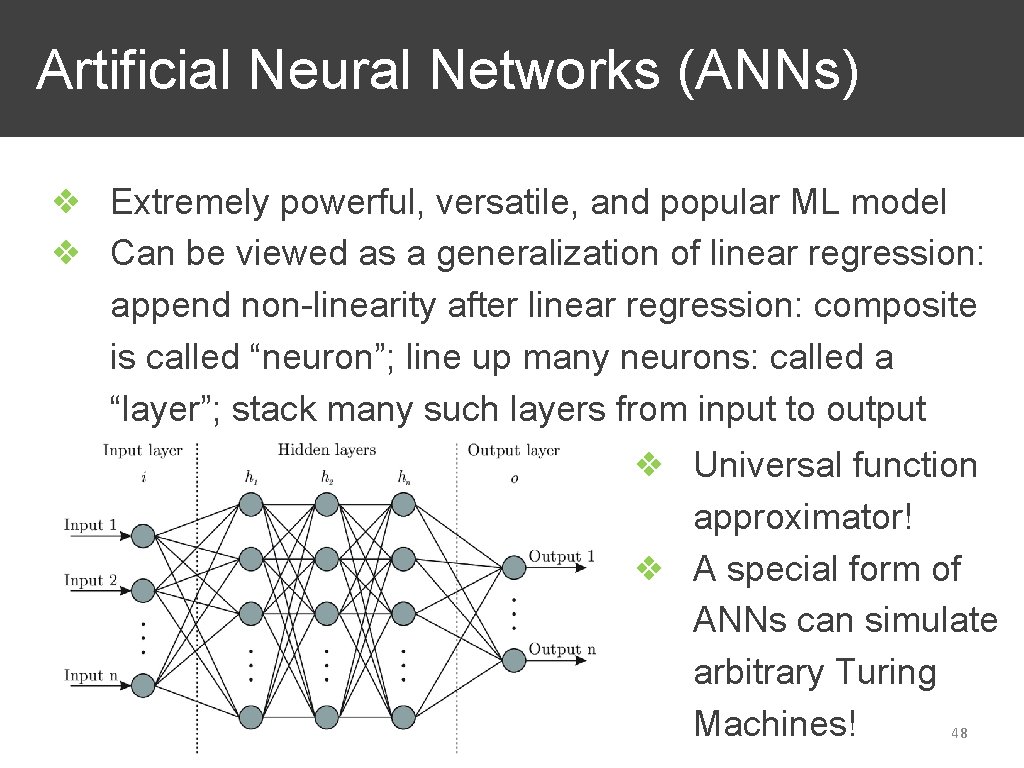
Artificial Neural Networks (ANNs) ❖ Extremely powerful, versatile, and popular ML model ❖ Can be viewed as a generalization of linear regression: append non-linearity after linear regression: composite is called “neuron”; line up many neurons: called a “layer”; stack many such layers from input to output ❖ Universal function approximator! ❖ A special form of ANNs can simulate arbitrary Turing Machines! 48

Artificial Neural Networks (ANNs) ❖ Different forms of ANNs tailored for different “raw” data representations for input and/or output ❖ Multi-Layer Perceptrons (MLPs) deal with a “flat” numeric vector for input and/or output ❖ Recurrent Neural Networks (RNNs) tailored for sequentially structured inputs (text, time series, etc. ), Convolutional Neural Networks (CNNs) for images/spatially structured data, etc. ❖ Bottomline: ANNs can help approximate any function! 49 (Switch to Tim Kraska’s slides)

Sorting: Outline ❖ Overview and Warm-up ❖ Multi-way External Merge Sort (EMS) ❖ EMS and B+ trees 50

Motivation for Sorting ❖ User’s SQL query has ORDER BY clause! ❖ First step of bulk loading of a B+ tree index ❖ Used in implementations of many relational ops: project, join, set ops, group by aggregate, etc. (next topic!) Q: But sorting is well-known; why should a DBMS bother? Often, the file (relation) to be sorted will not fit in RAM! “External” Sorting 51

External Sorting: Overview ❖ Goal: Given relation R with N pages, Sort. Key A, M buffer pages (often, M << N), sort R on A to get sorted R’ ❖ Idea: Sorting algorithm should be disk page I/O-aware! ❖ Desiderata: ❖ High efficiency, i. e. , low I/O cost, even for very large N ❖ Use sequential I/Os rather than random I/Os AMAP ❖ Interleave I/O and comp. (DMA); reduce CPU cost too NB: I/O-aware sorting is also a key part of the implementation of Map. Reduce/Hadoop! 52

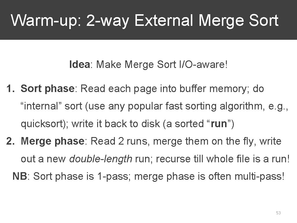
Warm-up: 2 -way External Merge Sort Idea: Make Merge Sort I/O-aware! 1. Sort phase: Read each page into buffer memory; do “internal” sort (use any popular fast sorting algorithm, e. g. , quicksort); write it back to disk (a sorted “run”) 2. Merge phase: Read 2 runs, merge them on the fly, write out a new double-length run; recurse till whole file is a run! NB: Sort phase is 1 -pass; merge phase is often multi-pass! 53

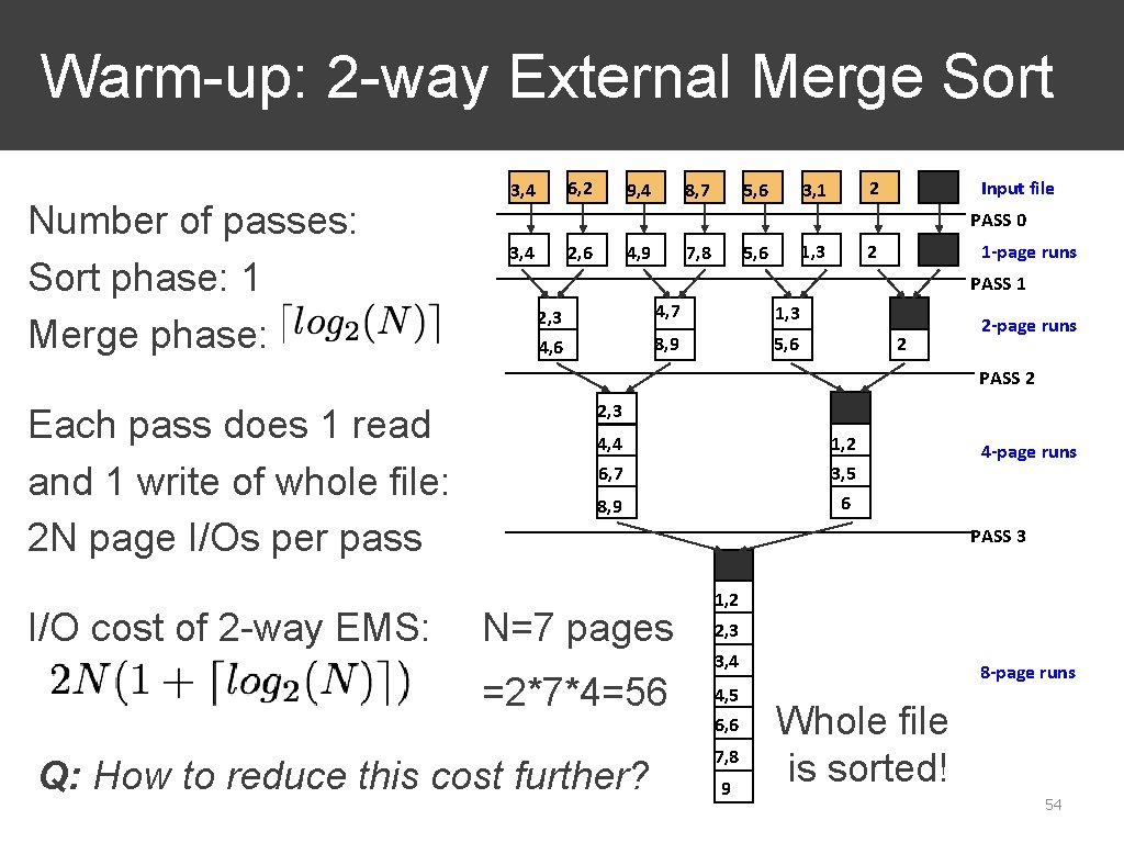
Warm-up: 2 -way External Merge Sort Number of passes: Sort phase: 1 Merge phase: 6, 2 3, 4 9, 4 8, 7 5, 6 2 3, 1 Input file PASS 0 3, 4 2, 6 4, 9 7, 8 1, 3 5, 6 2 1 -page runs PASS 1 2, 3 4, 7 1, 3 4, 6 8, 9 5, 6 2 2 -page runs PASS 2 Each pass does 1 read and 1 write of whole file: 2 N page I/Os per pass I/O cost of 2 -way EMS: 2, 3 4, 4 1, 2 6, 7 3, 5 6 8, 9 4 -page runs PASS 3 N=7 pages =2*7*4=56 Q: How to reduce this cost further? 1, 2 2, 3 3, 4 4, 5 6, 6 7, 8 9 8 -page runs Whole file is sorted! 54

Sorting: Outline ❖ Overview and Warm-up ❖ Multi-way External Merge Sort (EMS) ❖ EMS and B+ trees 55

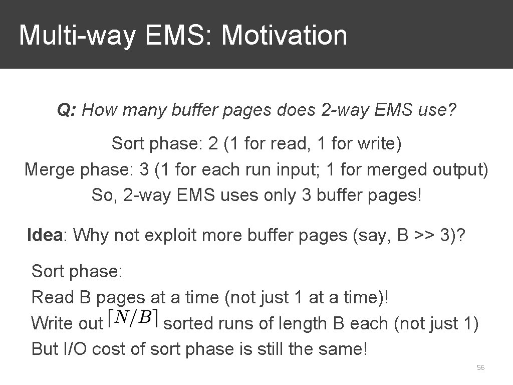
Multi-way EMS: Motivation Q: How many buffer pages does 2 -way EMS use? Sort phase: 2 (1 for read, 1 for write) Merge phase: 3 (1 for each run input; 1 for merged output) So, 2 -way EMS uses only 3 buffer pages! Idea: Why not exploit more buffer pages (say, B >> 3)? Sort phase: Read B pages at a time (not just 1 at a time)! Write out sorted runs of length B each (not just 1) But I/O cost of sort phase is still the same! 56

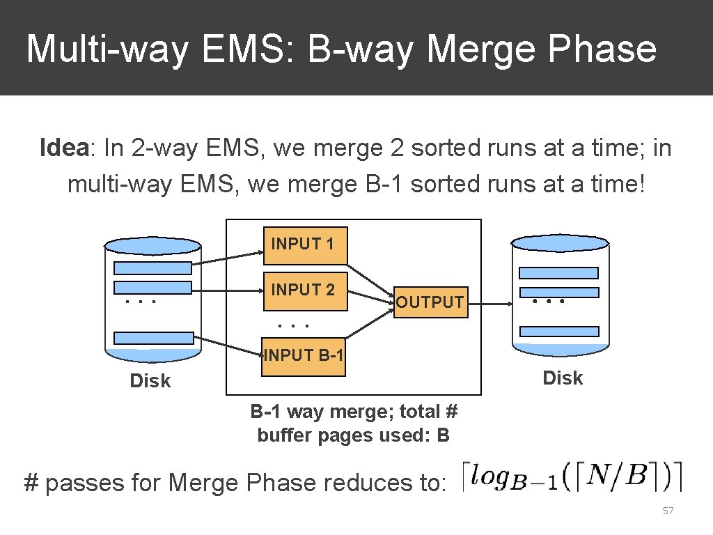
Multi-way EMS: B-way Merge Phase Idea: In 2 -way EMS, we merge 2 sorted runs at a time; in multi-way EMS, we merge B-1 sorted runs at a time! INPUT 1 . . . INPUT 2 . . . OUTPUT . . . INPUT B-1 Disk B-1 way merge; total # buffer pages used: B # passes for Merge Phase reduces to: 57

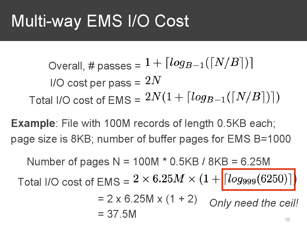
Multi-way EMS I/O Cost Overall, # passes = I/O cost per pass = Total I/O cost of EMS = Example: File with 100 M records of length 0. 5 KB each; page size is 8 KB; number of buffer pages for EMS B=1000 Number of pages N = 100 M * 0. 5 KB / 8 KB = 6. 25 M Total I/O cost of EMS = = 2 x 6. 25 M x (1 + 2) = 37. 5 M Only need the ceil! 58

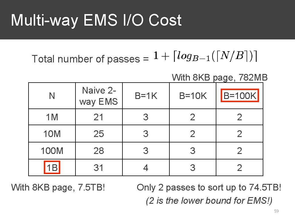
Multi-way EMS I/O Cost Total number of passes = With 8 KB page, 782 MB N Naive 2 way EMS B=1 K B=100 K 1 M 21 3 2 2 10 M 25 3 2 2 100 M 28 3 3 2 1 B 31 4 3 2 With 8 KB page, 7. 5 TB! Only 2 passes to sort up to 74. 5 TB! (2 is the lower bound for EMS!) 59

Multi-way EMS: Improvements ❖ While already efficient, some key algorithmic+systemsoriented improvements have been made to multi-way EMS to reduce overall runtime (not just counting I/O cost) ❖ Three prominent improvements: 1. Replacement sort (aka heap sort) as internal sort 2. “Blocked” I/O 3. Double Buffering 60

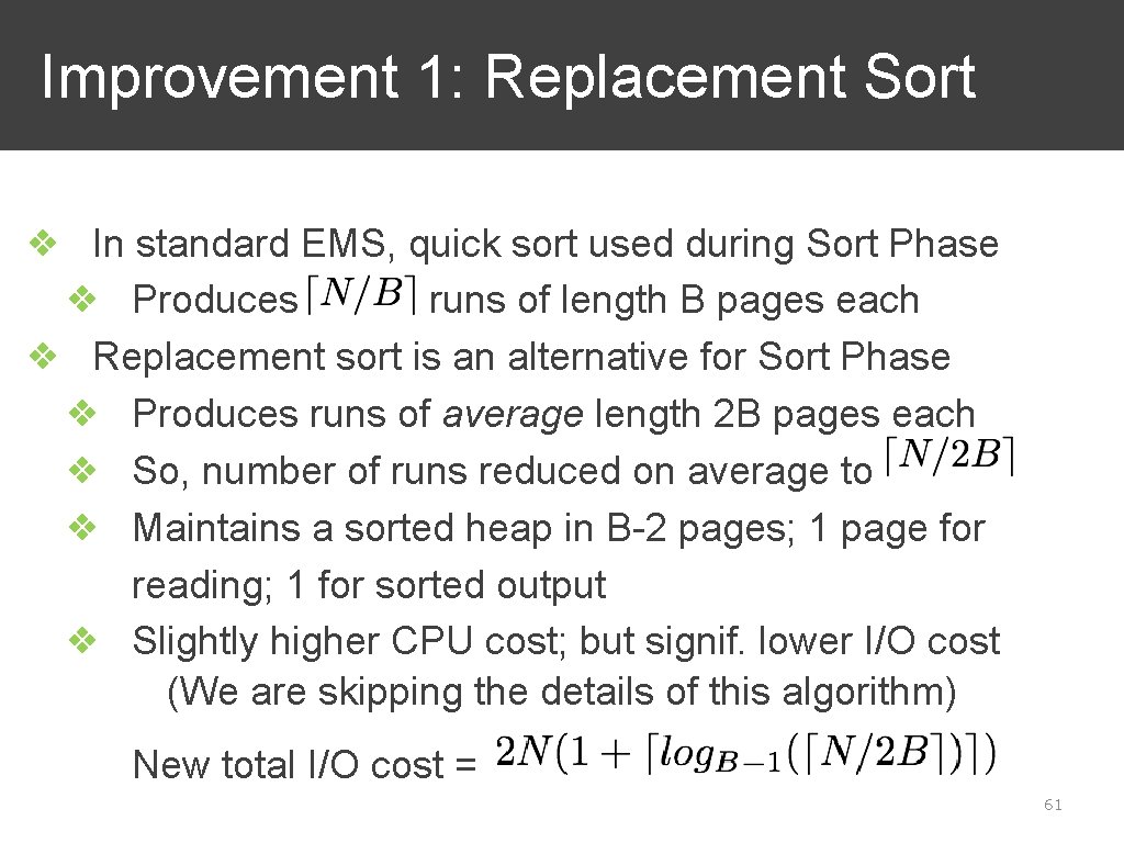
Improvement 1: Replacement Sort ❖ In standard EMS, quick sort used during Sort Phase ❖ Produces runs of length B pages each ❖ Replacement sort is an alternative for Sort Phase ❖ Produces runs of average length 2 B pages each ❖ So, number of runs reduced on average to ❖ Maintains a sorted heap in B-2 pages; 1 page for reading; 1 for sorted output ❖ Slightly higher CPU cost; but signif. lower I/O cost (We are skipping the details of this algorithm) New total I/O cost = 61

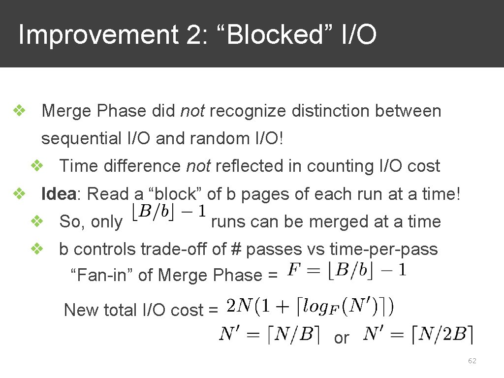
Improvement 2: “Blocked” I/O ❖ Merge Phase did not recognize distinction between sequential I/O and random I/O! ❖ Time difference not reflected in counting I/O cost ❖ Idea: Read a “block” of b pages of each run at a time! ❖ So, only runs can be merged at a time ❖ b controls trade-off of # passes vs time-per-pass “Fan-in” of Merge Phase = New total I/O cost = or 62

Improvement 3: Double Buffering ❖ Most machines have DMA; enables I/O-CPU parallelism ❖ Trivially feasible to exploit DMA in the Sort Phase ❖ But in the Merge Phase, CPU blocked by I/O for runs ❖ Idea: Allocate double the buffers for each run; while CPU processes one set, read pages (I/O) into other set! ❖ So, only runs can be merged at a time New fan-in of Merge Phase = F = New total I/O cost = or 63

Sorting: Outline ❖ Overview and Warm-up ❖ Multi-way External Merge Sort (EMS) ❖ EMS and B+ trees 64

Using B+ Tree for EMS ❖ Suppose we already have a B+ tree index with the Sort. Key being equal to (or a prefix of) the Index. Key ❖ Data entries of the B+ tree are already in sorted order! Q: Is it a “good” idea to simply read the leaf level of the B+ tree to achieve the EMS then? It depends! On whether the index is clustered or not! Good idea! Might be really bad! 65

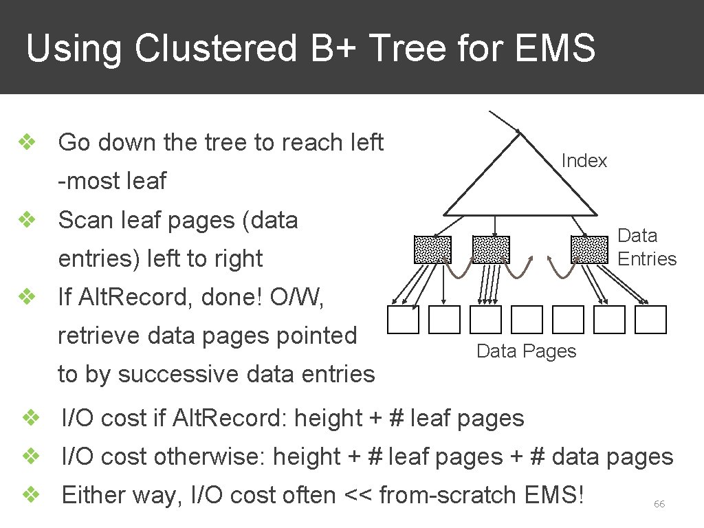
Using Clustered B+ Tree for EMS ❖ Go down the tree to reach left Index -most leaf ❖ Scan leaf pages (data Data Entries entries) left to right ❖ If Alt. Record, done! O/W, retrieve data pages pointed to by successive data entries Data Pages ❖ I/O cost if Alt. Record: height + # leaf pages ❖ I/O cost otherwise: height + # leaf pages + # data pages ❖ Either way, I/O cost often << from-scratch EMS! 66

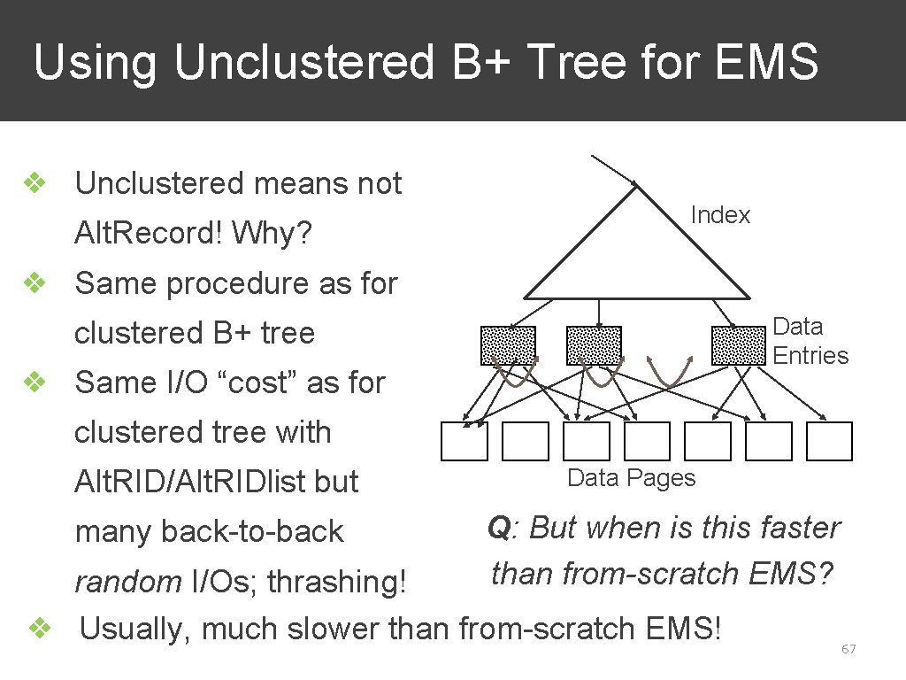
Using Unclustered B+ Tree for EMS ❖ Unclustered means not Alt. Record! Why? Index ❖ Same procedure as for Data Entries clustered B+ tree ❖ Same I/O “cost” as for clustered tree with Alt. RID/Alt. RIDlist but many back-to-back Data Pages Q: But when is this faster than from-scratch EMS? random I/Os; thrashing! ❖ Usually, much slower than from-scratch EMS! 67

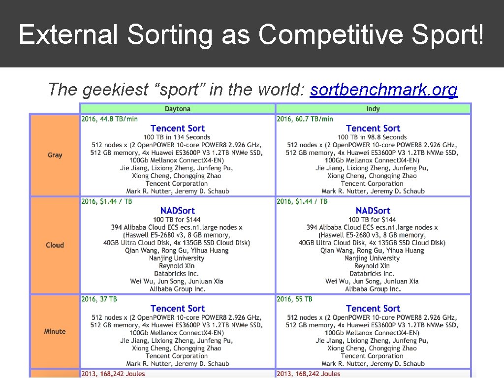
External Sorting as Competitive Sport! The geekiest “sport” in the world: sortbenchmark. org 68