CSE 202 Algorithms Quicksort vs Heapsort the official

CSE 202 - Algorithms • Quicksort vs Heapsort: • the “official” story • Next time, we’ll get the “inside” story! 4/10/2003 CSE 202 - Quick&Heap

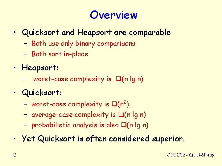
Overview • Quicksort and Heapsort are comparable – Both use only binary comparisons – Both sort in-place • Heapsort: – worst-case complexity is (n lg n) • Quicksort: – worst-case complexity is (n 2). – average-case complexity is (n lg n) – probabilistic analysis is also (n lg n) • Yet Quicksort is often considered superior. 2 CSE 202 - Quick&Heap

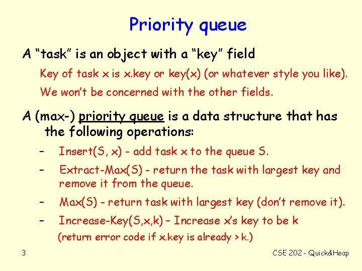
Priority queue A “task” is an object with a “key” field Key of task x is x. key or key(x) (or whatever style you like). We won’t be concerned with the other fields. A (max-) priority queue is a data structure that has the following operations: – Insert(S, x) - add task x to the queue S. – Extract-Max(S) - return the task with largest key and remove it from the queue. – Max(S) - return task with largest key (don’t remove it). – Increase-Key(S, x, k) – Increase x’s key to be k (return error code if x. key is already > k. ) 3 CSE 202 - Quick&Heap

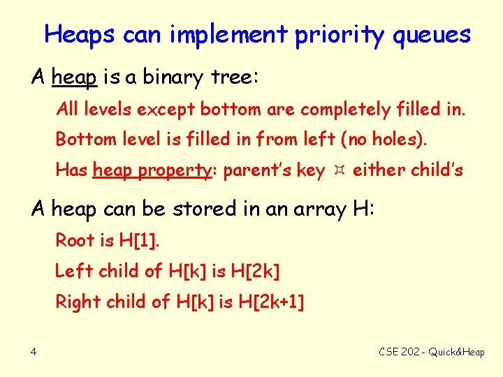
Heaps can implement priority queues A heap is a binary tree: All levels except bottom are completely filled in. Bottom level is filled in from left (no holes). Has heap property: parent’s key either child’s A heap can be stored in an array H: Root is H[1]. Left child of H[k] is H[2 k] Right child of H[k] is H[2 k+1] 4 CSE 202 - Quick&Heap

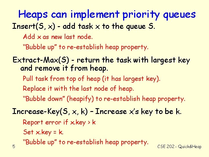
Heaps can implement priority queues Insert(S, x) - add task x to the queue S. Add x as new last node. “Bubble up” to re-establish heap property. Extract-Max(S) - return the task with largest key and remove it from heap. Pull task from top of heap (it has largest key). Replace it with the last node of heap. “Bubble down” (heapify) to re-establish heap property. Increase-Key(S, x, k) – Increase x’s key to be k. Report error if x. key > k Set x. key = k. 5 “Bubble up” to re-establish heap property. CSE 202 - Quick&Heap

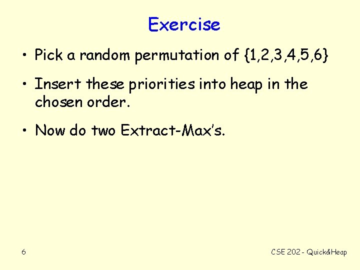
Exercise • Pick a random permutation of {1, 2, 3, 4, 5, 6} • Insert these priorities into heap in the chosen order. • Now do two Extract-Max’s. 6 CSE 202 - Quick&Heap

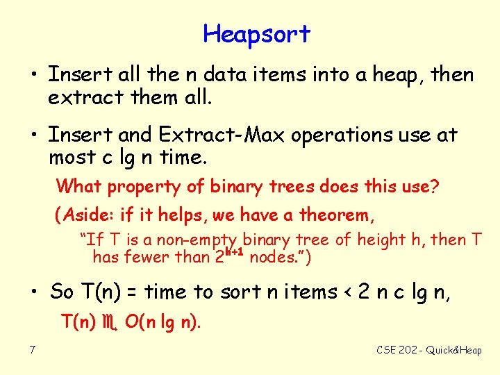
Heapsort • Insert all the n data items into a heap, then extract them all. • Insert and Extract-Max operations use at most c lg n time. What property of binary trees does this use? (Aside: if it helps, we have a theorem, “If T is a non-empty binary tree of height h, then T has fewer than 2 h+1 nodes. ”) • So T(n) = time to sort n items < 2 n c lg n, T(n) O(n lg n). 7 CSE 202 - Quick&Heap

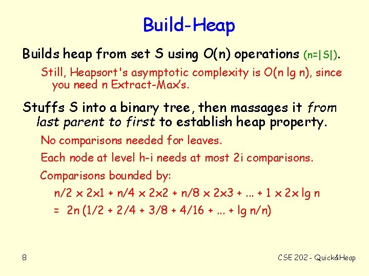
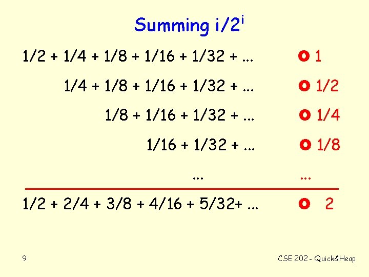
Build-Heap Builds heap from set S using O(n) operations (n=|S|). Still, Heapsort's asymptotic complexity is O(n lg n), since you need n Extract-Max’s. Stuffs S into a binary tree, then massages it from last parent to first to establish heap property. No comparisons needed for leaves. Each node at level h-i needs at most 2 i comparisons. Comparisons bounded by: n/2 x 2 x 1 + n/4 x 2 x 2 + n/8 x 2 x 3 +. . . + 1 x 2 x lg n = 2 n (1/2 + 2/4 + 3/8 + 4/16 +. . . + lg n/n) 8 CSE 202 - Quick&Heap

Summing i/2 i 1/2 + 1/4 + 1/8 + 1/16 + 1/32 +. . . 1 1/4 + 1/8 + 1/16 + 1/32 +. . . 1/2 1/8 + 1/16 + 1/32 +. . . 1/4 1/16 + 1/32 +. . . 1/8 . . . 1/2 + 2/4 + 3/8 + 4/16 + 5/32+. . . 9 2 CSE 202 - Quick&Heap

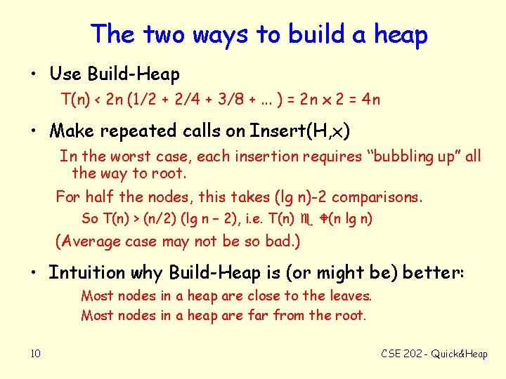
The two ways to build a heap • Use Build-Heap T(n) < 2 n (1/2 + 2/4 + 3/8 +. . . ) = 2 n x 2 = 4 n • Make repeated calls on Insert(H, x) In the worst case, each insertion requires “bubbling up” all the way to root. For half the nodes, this takes (lg n)-2 comparisons. So T(n) > (n/2) (lg n – 2), i. e. T(n) (n lg n) (Average case may not be so bad. ) • Intuition why Build-Heap is (or might be) better: Most nodes in a heap are close to the leaves. Most nodes in a heap are far from the root. 10 CSE 202 - Quick&Heap

Basic idea: Quicksort Split w. r. t A[1] Arrange A as: small elements ( A[1]) big ( A[1]) A[1] Recursively arrange “small” part and “big” parts. Doesn’t need extra array. Keep pointers to current ends of small & big parts. small unpartitioned big “Pick up” A[1] (splitter) and A[n] (current element), 11 leaves space in to deposit element in either part drop current element appropriately; pick up next innermost. CSE 202 - Quick&Heap

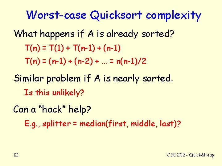
Worst-case Quicksort complexity What happens if A is already sorted? T(n) = T(1) + T(n-1) + (n-1) T(n) = (n-1) + (n-2) +. . . = n(n-1)/2 Similar problem if A is nearly sorted. Is this unlikely? Can a “hack” help? E. g. , splitter = median(first, middle, last)? 12 CSE 202 - Quick&Heap

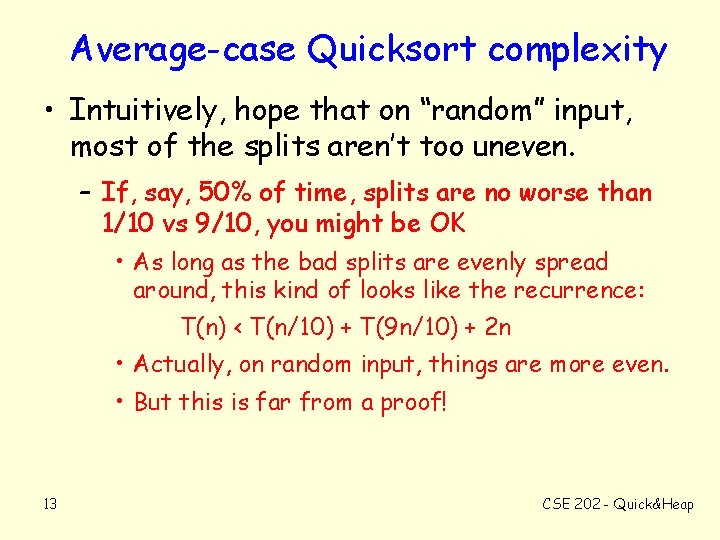
Average-case Quicksort complexity • Intuitively, hope that on “random” input, most of the splits aren’t too uneven. – If, say, 50% of time, splits are no worse than 1/10 vs 9/10, you might be OK • As long as the bad splits are evenly spread around, this kind of looks like the recurrence: T(n) < T(n/10) + T(9 n/10) + 2 n • Actually, on random input, things are more even. • But this is far from a proof! 13 CSE 202 - Quick&Heap

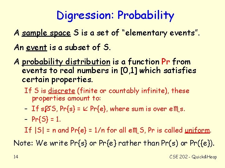
Digression: Probability A sample space S is a set of “elementary events”. An event is a subset of S. A probability distribution is a function Pr from events to real numbers in [0, 1] which satisfies certain properties. If S is discrete (finite or countably infinite), these properties amount to: – If s S, Pr{s} = Pr{e}, where sum is over e s. – Pr{S} = 1. If |S| = n and Pr{e} = 1/n for all e S, Pr is called uniform. Note: We write Pr{s} or Pr{e} rather than Pr(s) or Pr({e}). 14 CSE 202 - Quick&Heap

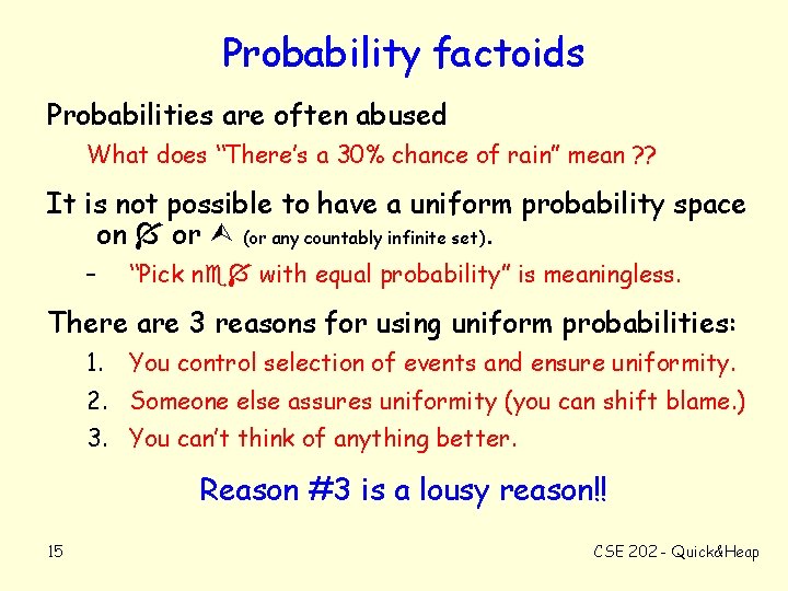
Probability factoids Probabilities are often abused What does “There’s a 30% chance of rain” mean ? ? It is not possible to have a uniform probability space on or (or any countably infinite set). – “Pick n with equal probability” is meaningless. There are 3 reasons for using uniform probabilities: 1. You control selection of events and ensure uniformity. 2. Someone else assures uniformity (you can shift blame. ) 3. You can’t think of anything better. Reason #3 is a lousy reason!! 15 CSE 202 - Quick&Heap

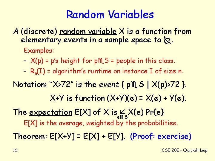
Random Variables A (discrete) random variable X is a function from elementary events in a sample space to . Examples: – X(p) = p’s height for p S = people in this class. – Rn(I) = algorithm’s runtime on instance I of size n. Notation: “X>72” is the event { p S | X(p)>72 }. X+Y is function (X+Y)(e) = X(e) + Y(e). The expectation E[X] of X ise S X(e) Pr{e} E[X] is the average, weighted by the probabilities. Theorem: E[X+Y] = E[X] + E[Y]. (Proof: exercise) 16 CSE 202 - Quick&Heap

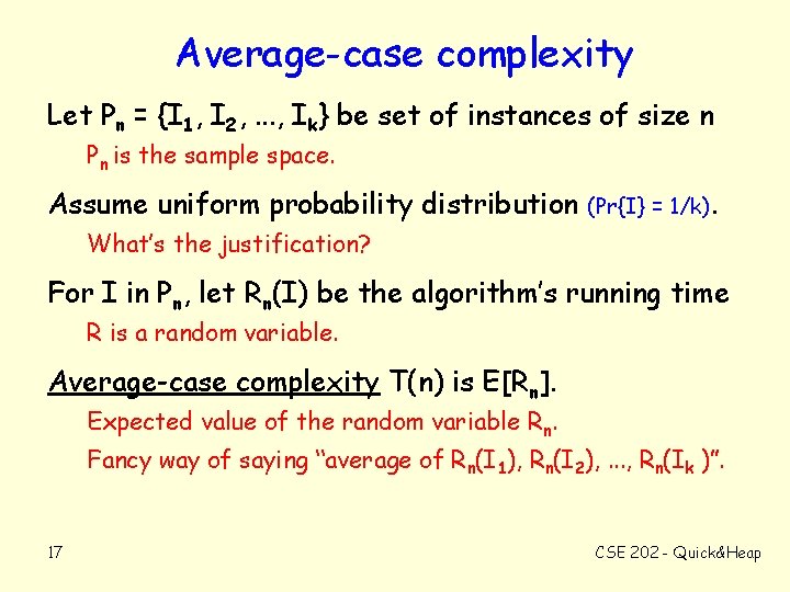
Average-case complexity Let Pn = {I 1, I 2, . . . , Ik} be set of instances of size n Pn is the sample space. Assume uniform probability distribution (Pr{I} = 1/k). What’s the justification? For I in Pn, let Rn(I) be the algorithm’s running time R is a random variable. Average-case complexity T(n) is E[Rn]. Expected value of the random variable Rn. Fancy way of saying “average of Rn(I 1), Rn(I 2), . . . , Rn(Ik )”. 17 CSE 202 - Quick&Heap

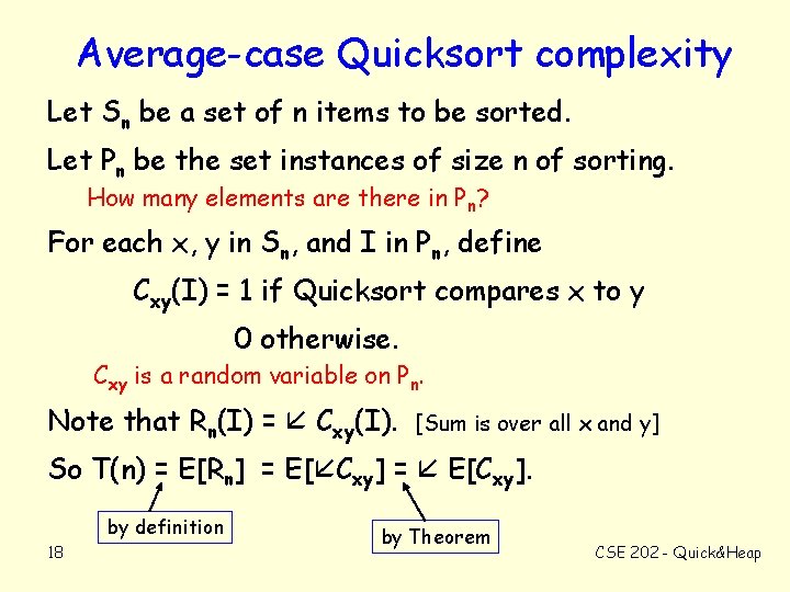
Average-case Quicksort complexity Let Sn be a set of n items to be sorted. Let Pn be the set instances of size n of sorting. How many elements are there in Pn? For each x, y in Sn, and I in Pn, define Cxy(I) = 1 if Quicksort compares x to y 0 otherwise. Cxy is a random variable on Pn. Note that Rn(I) = Cxy(I). [Sum is over all x and y] So T(n) = E[Rn] = E[ Cxy] = E[Cxy]. by definition 18 by Theorem CSE 202 - Quick&Heap

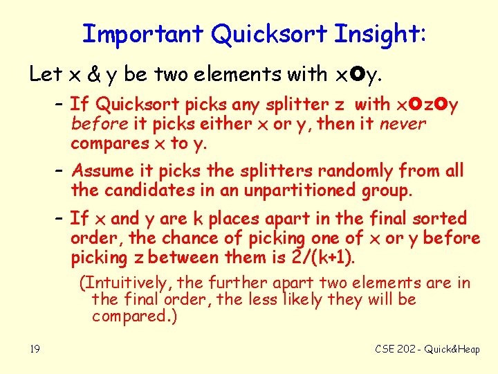
Important Quicksort Insight: Let x & y be two elements with x y. – If Quicksort picks any splitter z with x z y before it picks either x or y, then it never compares x to y. – Assume it picks the splitters randomly from all the candidates in an unpartitioned group. – If x and y are k places apart in the final sorted order, the chance of picking one of x or y before picking z between them is 2/(k+1). (Intuitively, the further apart two elements are in the final order, the less likely they will be compared. ) 19 CSE 202 - Quick&Heap

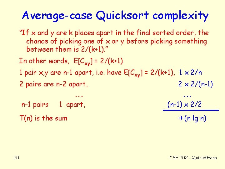
Average-case Quicksort complexity “If x and y are k places apart in the final sorted order, the chance of picking one of x or y before picking something between them is 2/(k+1). ” In other words, E[Cxy] = 2/(k+1) 1 pair x, y are n-1 apart, i. e. have E[Cxy] = 2/(k+1), 1 x 2/n 2 pairs are n-2 apart, . . . n-1 pairs 1 apart, T(n) is the sum 20 2 x 2/(n-1). . . (n-1) x 2/2 (n lg n) CSE 202 - Quick&Heap

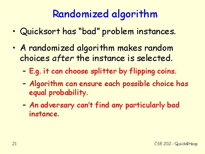
Randomized algorithm • Quicksort has “bad” problem instances. • A randomized algorithm makes random choices after the instance is selected. – E. g. it can choose splitter by flipping coins. – Algorithm can ensure each possible choice has equal probability. – An adversary can’t find any particularly bad instance. 21 CSE 202 - Quick&Heap

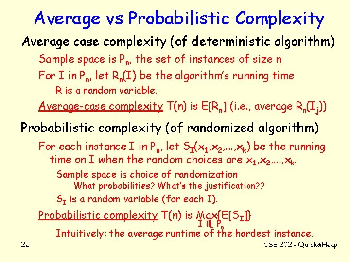
Average vs Probabilistic Complexity Average case complexity (of deterministic algorithm) Sample space is Pn, the set of instances of size n For I in Pn, let Rn(I) be the algorithm’s running time R is a random variable. Average-case complexity T(n) is E[Rn] (i. e. , average Rn(Ij)) Probabilistic complexity (of randomized algorithm) For each instance I in Pn, let SI(x 1, x 2, . . . , xk) be the running time on I when the random choices are x 1, x 2, . . . , xk. Sample space is choice of randomization What probabilities? What’s the justification? ? SI is a random variable (for each I). Probabilistic complexity T(n) is Max{E[SI]} I Pn 22 Intuitively: the average runtime of the hardest instance. CSE 202 - Quick&Heap

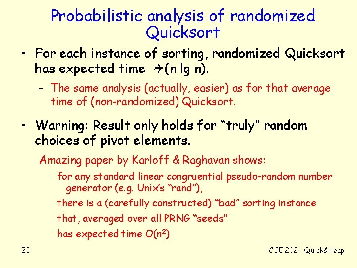
Probabilistic analysis of randomized Quicksort • For each instance of sorting, randomized Quicksort has expected time (n lg n). – The same analysis (actually, easier) as for that average time of (non-randomized) Quicksort. • Warning: Result only holds for “truly” random choices of pivot elements. Amazing paper by Karloff & Raghavan shows: for any standard linear congruential pseudo-random number generator (e. g. Unix’s “rand”), there is a (carefully constructed) “bad” sorting instance that, averaged over all PRNG “seeds” has expected time O(n 2) 23 CSE 202 - Quick&Heap

Why use Quicksort? • “Quicksort has tight code, so the hidden constant factor in its running time is small” (Text, pg 125). – Doesn’t Heapsort also? ? • “[Quicksort] works well even in virtual memory environments. ” (Text, pg 145). – We’ll see what that means! 24 CSE 202 - Quick&Heap

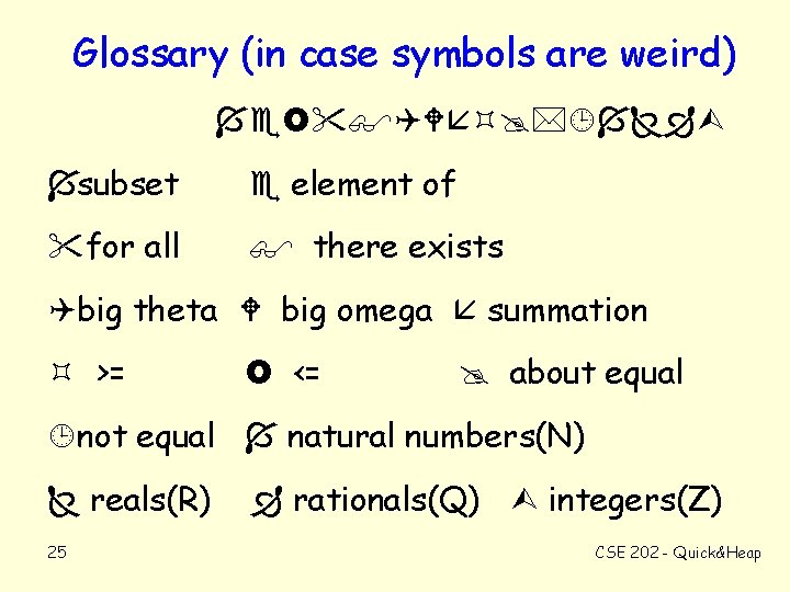
Glossary (in case symbols are weird) subset element of for all there exists big theta big omega summation >= <= about equal not equal natural numbers(N) reals(R) 25 rationals(Q) integers(Z) CSE 202 - Quick&Heap