CSE 1342 Programming Concepts Algorithmic Analysis Using BigO

CSE 1342 Programming Concepts Algorithmic Analysis Using Big-O Part 1

The Running Time of Programs n Most problems can be solved by more than one algorithm. So, how do you choose the best solution? n The best solution is usually based on efficiency n Efficiency of time (speed of execution) n Efficiency of space (memory usage) n In the case of a program that is infrequently run or subject to frequent modification, algorithmic simplicity may take precedence over efficiency.

The Running Time of Programs n An absolute measure of time (5. 3 seconds, for example) is not a practical measure of efficiency because … n The execution time is a function of the amount of data that the program manipulates and typically grows as the amount of data increases. n Different computers will execute the same program (using the same data) at different speeds. n Depending on the choice of programming language and compiler, speeds can vary on the same computer.

The Running Time of Programs n The solution is to remove all implementation considerations from our analysis and focus on those aspects of the algorithm that most critically effect the execution time. n The most important aspect is usually the number of data elements (n) the program must manipulate. n Occasionally the magnitude of a single data element (and not the number of data elements) is the most important aspect.

The 90 - 10 Rule n The 90 - 10 rule states that, in general, a program spends 90% of its time executing the same 10% of its code. n This is due to the fact that most programs rely heavily on repetition structures (loops and recursive calls). n Because of the 90 - 10 rule, algorithmic analysis focuses on repetition structures.

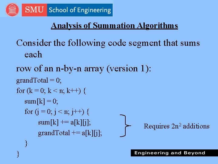
Analysis of Summation Algorithms Consider the following code segment that sums each row of an n-by-n array (version 1): grand. Total = 0; for (k = 0; k < n; k++) { sum[k] = 0; for (j = 0; j < n; j++) { sum[k] += a[k][j]; grand. Total += a[k][j]; } } Requires 2 n 2 additions

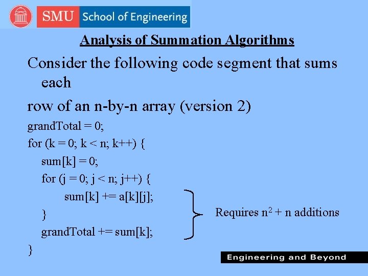
Analysis of Summation Algorithms Consider the following code segment that sums each row of an n-by-n array (version 2) grand. Total = 0; for (k = 0; k < n; k++) { sum[k] = 0; for (j = 0; j < n; j++) { sum[k] += a[k][j]; } grand. Total += sum[k]; } Requires n 2 + n additions

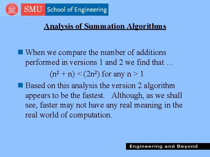
Analysis of Summation Algorithms n When we compare the number of additions performed in versions 1 and 2 we find that … (n 2 + n) < (2 n 2) for any n > 1 n Based on this analysis the version 2 algorithm appears to be the fastest. Although, as we shall see, faster may not have any real meaning in the real world of computation.

Analysis of Summation Algorithms n Further analysis of the two summation algorithms. n Assume a 1000 by 1000 ( n = 1000) array and a computer that can execute an addition instruction in 1 microsecond. • 1 microsecond = one millionth of a second. n n n The version 1 algorithm (2 n 2) would require 2(10002)/1, 000 = 2 seconds to execute. The version 2 algorithm (n 2 + n) would require (10002 + 1000)/1, 000 = = 1. 001 seconds to execute. From a users real-time perspective the difference is insignificant

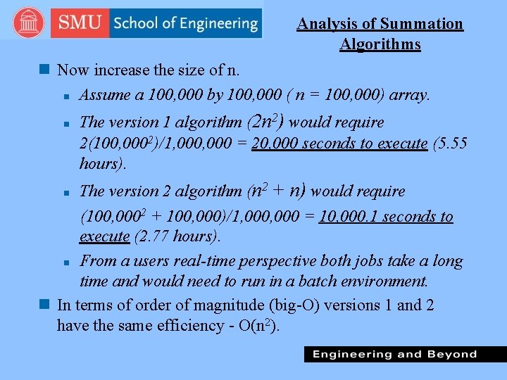
Analysis of Summation Algorithms n Now increase the size of n. n Assume a 100, 000 by 100, 000 ( n = 100, 000) array. n The version 1 algorithm (2 n 2) would require 2(100, 0002)/1, 000 = 20, 000 seconds to execute (5. 55 hours). The version 2 algorithm (n 2 + n) would require (100, 0002 + 100, 000)/1, 000 = 10, 000. 1 seconds to execute (2. 77 hours). n From a users real-time perspective both jobs take a long time and would need to run in a batch environment. n In terms of order of magnitude (big-O) versions 1 and 2 have the same efficiency - O(n 2). n

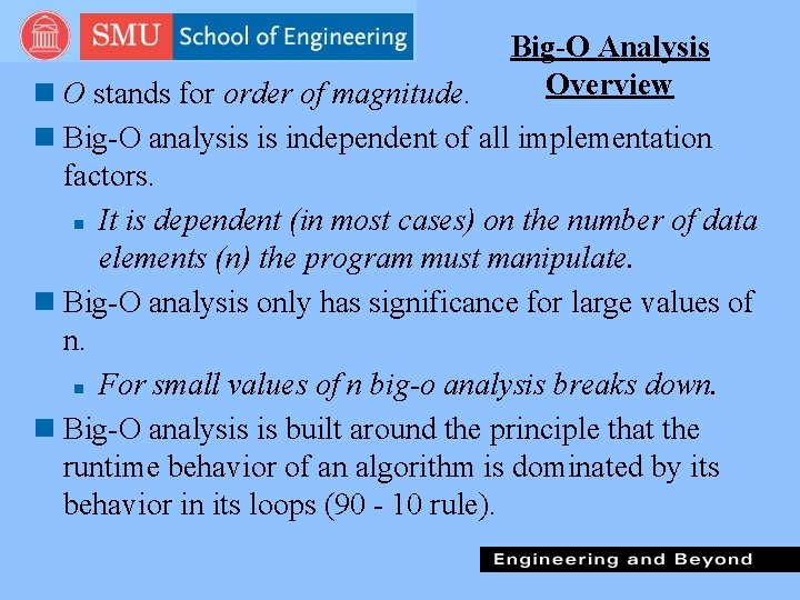
Big-O Analysis Overview n O stands for order of magnitude. n Big-O analysis is independent of all implementation factors. n It is dependent (in most cases) on the number of data elements (n) the program must manipulate. n Big-O analysis only has significance for large values of n. n For small values of n big-o analysis breaks down. n Big-O analysis is built around the principle that the runtime behavior of an algorithm is dominated by its behavior in its loops (90 - 10 rule).

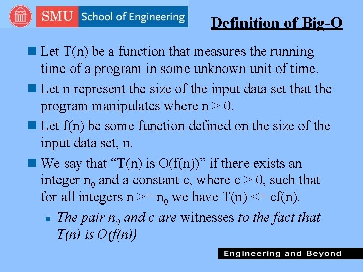
Definition of Big-O n Let T(n) be a function that measures the running time of a program in some unknown unit of time. n Let n represent the size of the input data set that the program manipulates where n > 0. n Let f(n) be some function defined on the size of the input data set, n. n We say that “T(n) is O(f(n))” if there exists an integer n 0 and a constant c, where c > 0, such that for all integers n >= n 0 we have T(n) <= cf(n). n The pair n 0 and c are witnesses to the fact that T(n) is O(f(n))

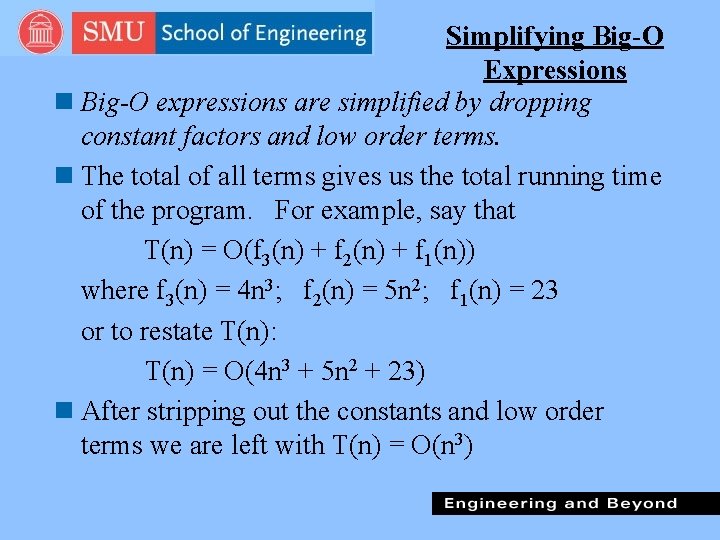
Simplifying Big-O Expressions n Big-O expressions are simplified by dropping constant factors and low order terms. n The total of all terms gives us the total running time of the program. For example, say that T(n) = O(f 3(n) + f 2(n) + f 1(n)) where f 3(n) = 4 n 3; f 2(n) = 5 n 2; f 1(n) = 23 or to restate T(n): T(n) = O(4 n 3 + 5 n 2 + 23) n After stripping out the constants and low order terms we are left with T(n) = O(n 3)

Simplifying Big-O Expressions T(n) = f 1(n) + f 2(n) + f 3(n) + … + fk(n) n In big-O analysis, one of the terms in the T(n) expression is identified as the dominant term. n A dominant term is one that, for large values of n, becomes so large that it allows us to ignore the other terms in the expression. n The problem of big-O analysis can be reduced to one of finding the dominant term in an expression representing the number of operations required by an algorithm. n All other terms and constants are dropped from the expression.

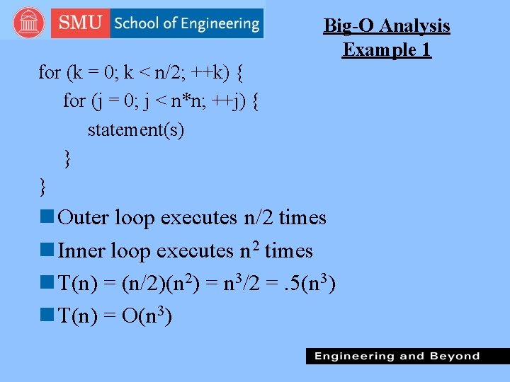
Big-O Analysis Example 1 for (k = 0; k < n/2; ++k) { for (j = 0; j < n*n; ++j) { statement(s) } } n Outer loop executes n/2 times n Inner loop executes n 2 times n T(n) = (n/2)(n 2) = n 3/2 =. 5(n 3) n T(n) = O(n 3)

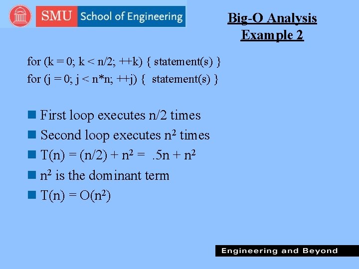
Big-O Analysis Example 2 for (k = 0; k < n/2; ++k) { statement(s) } for (j = 0; j < n*n; ++j) { statement(s) } n First loop executes n/2 times n Second loop executes n 2 times n T(n) = (n/2) + n 2 =. 5 n + n 2 n n 2 is the dominant term n T(n) = O(n 2)

Big-O Analysis Example 3 while (n > 1) { statement(s) n = n / 2; } n The values of n will follow a logarithmic progression. n Assuming n has the initial value of 64, the progression will be 64, 32, 16, 8, 4, 2. n Loop executes log 2 times n O(log 2 n) = O(log n)

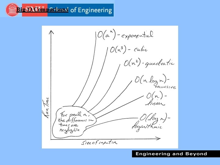
Big-O Comparisons

Analysis Involving if/else if (condition) loop 1; //assume O(f(n)) for loop 1 else loop 2; //assume O(g(n)) for loop 2 n The order of magnitude for the entire if/else statement is O(max(f(n), g(n)))

An Example Involving if/else if (a[1][1] = = 0) for (i = 0; i < n; ++i) for (j = 0; j < n; ++j) a[i][j] = 0; f(n) = n 2 else for (i = 0; i < n; ++i) a[i][j] = 1; g(n) = n n The order of magnitude for the entire if/else statement is O(max(f(n), g(n))) = O(n 2)