CSCI 631 Foundations of Computer Vision Ifeoma Nwogu

CSCI 631 Foundations of Computer Vision Ifeoma Nwogu ion@cs. rit. edu Lecture 16 – Convolutional neural networks

Schedule • Last class – Neural networks • Today – Convolutional neural networks I • Readings for today: – Online deep learning tutorial from Stanford http: //cs 231 n. github. io/convolutional-networks/ 2

Announcement • Talk by Christopher Kanan from Imaging Science: – Wednesday April 19, 2017; 1 pm in Liberal Arts Hall room 3225 • Title: Deep Machine Learning: Overview and Applications – Applications such as identifying people in photos, classifying objects in images, and playing board games, such as Go. – Technologies and computer hardware behind deep learning – Applications in which performance now rivals humans. – Ongoing work in his lab 3

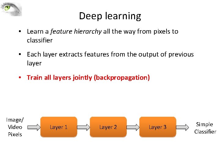
Deep learning • Learn a feature hierarchy all the way from pixels to classifier • Each layer extracts features from the output of previous layer • Train all layers jointly (backpropagation) Image/ Video Pixels Layer 1 Layer 2 Layer 3 Simple Classifier

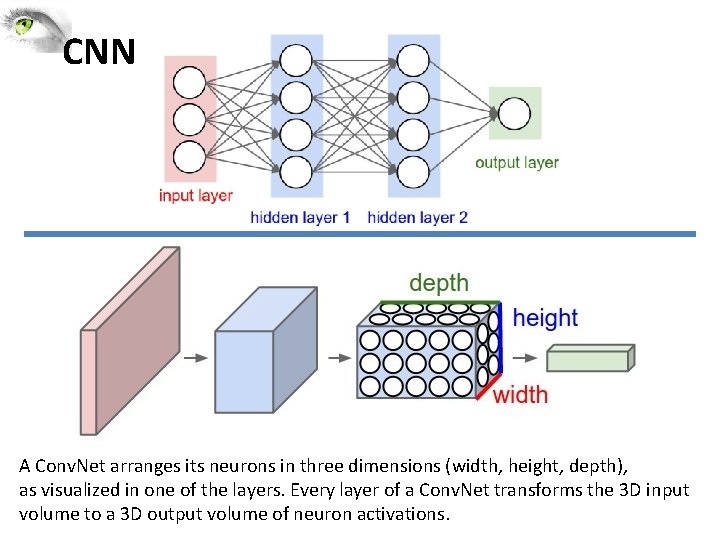
CNN A Conv. Net arranges its neurons in three dimensions (width, height, depth), as visualized in one of the layers. Every layer of a Conv. Net transforms the 3 D input volume to a 3 D output volume of neuron activations.

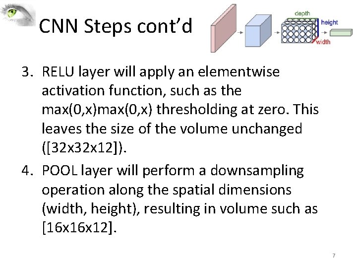
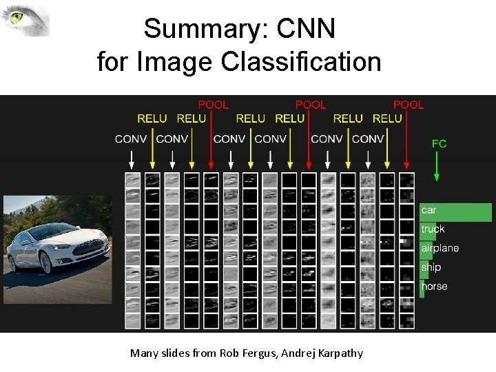
CNN Steps 1. INPUT [32 x 3] will hold the raw pixel values of the image, in this case an image of width 32, height 32, and with three color channels R, G, B. 2. CONV layer will compute the output of neurons that are connected to local regions in the input, each computing a dot product between their weights and a small region they are connected to in the input volume. This may result in volume such as [32 x 12] if we decided to use 12 filters. 6

CNN Steps cont’d 3. RELU layer will apply an elementwise activation function, such as the max(0, x) thresholding at zero. This leaves the size of the volume unchanged ([32 x 12]). 4. POOL layer will perform a downsampling operation along the spatial dimensions (width, height), resulting in volume such as [16 x 12]. 7

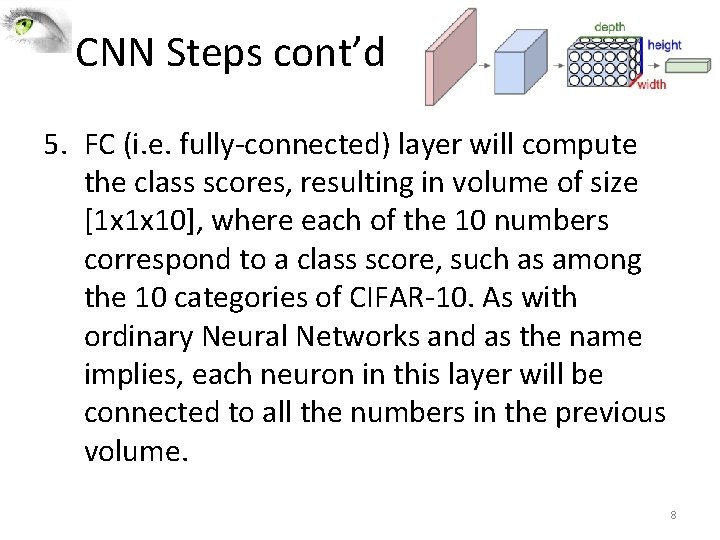
CNN Steps cont’d 5. FC (i. e. fully-connected) layer will compute the class scores, resulting in volume of size [1 x 1 x 10], where each of the 10 numbers correspond to a class score, such as among the 10 categories of CIFAR-10. As with ordinary Neural Networks and as the name implies, each neuron in this layer will be connected to all the numbers in the previous volume. 8

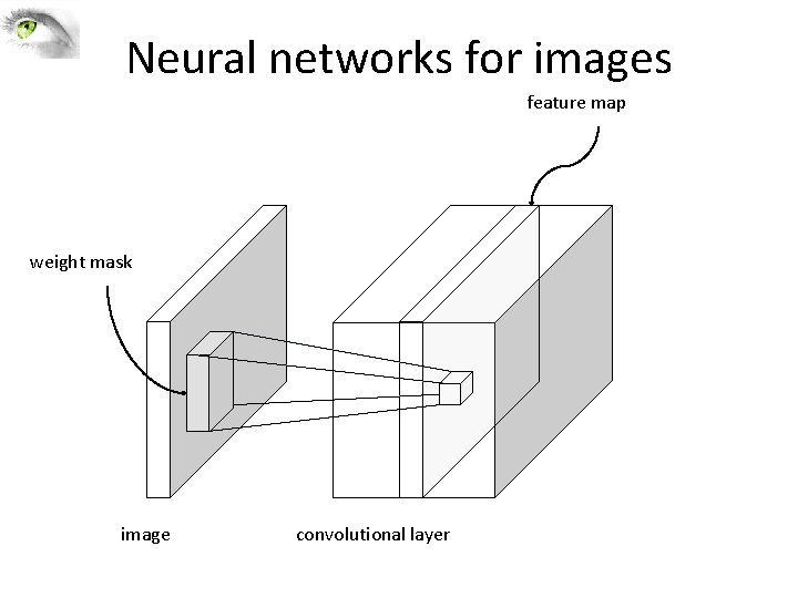
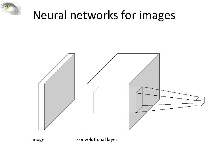
Neural networks for images feature map weight mask image convolutional layer

Neural networks for images image convolutional layer

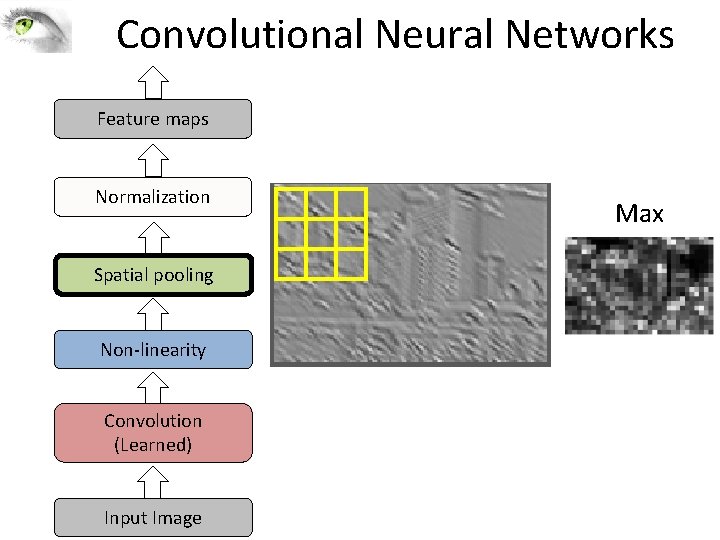
Pooling Input volume of size [224 x 64] is pooled with filter size 2, stride 2 into output volume of size [112 x 64]. 11

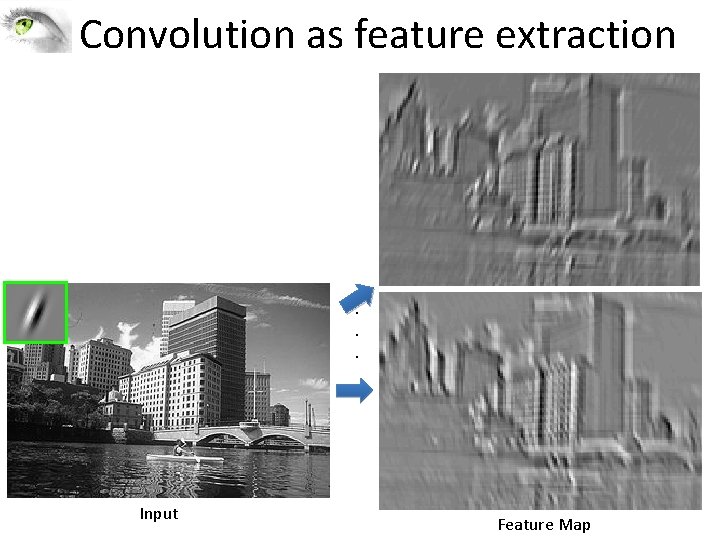
Convolution as feature extraction . . . Input Feature Map

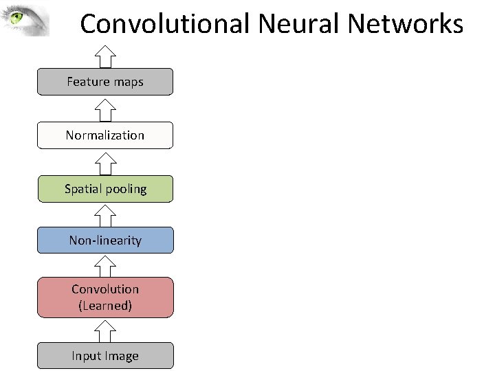
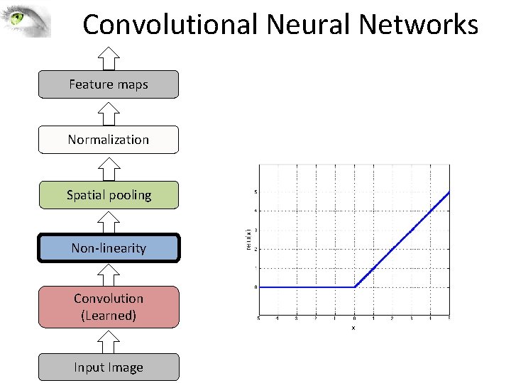
Convolutional Neural Networks Feature maps Normalization Spatial pooling Non-linearity Convolution (Learned) Input Image

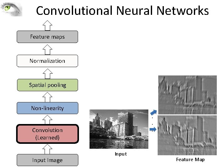
Convolutional Neural Networks Feature maps Normalization Spatial pooling Non-linearity. . . Convolution (Learned) Input Image Input Feature Map

Convolutional Neural Networks Feature maps Normalization Spatial pooling Non-linearity Convolution (Learned) Input Image

Convolutional Neural Networks Feature maps Normalization Spatial pooling Non-linearity Convolution (Learned) Input Image Max

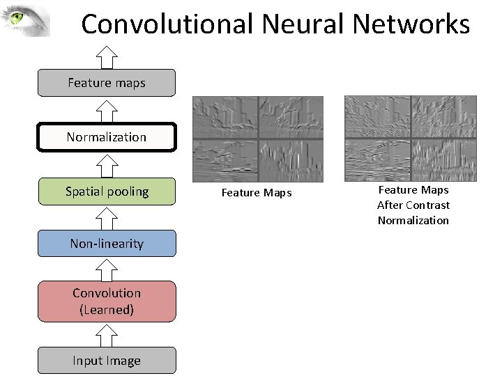
Convolutional Neural Networks Feature maps Normalization Spatial pooling Non-linearity Convolution (Learned) Input Image Feature Maps After Contrast Normalization

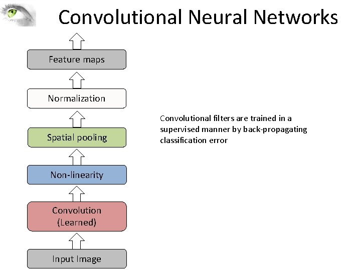
Convolutional Neural Networks Feature maps Normalization Spatial pooling Non-linearity Convolution (Learned) Input Image Convolutional filters are trained in a supervised manner by back-propagating classification error

Summary: CNN for Image Classification Many slides from Rob Fergus, Andrej Karpathy

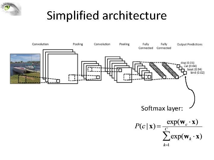
Simplified architecture Softmax layer:

Compare: SIFT Descriptor Image Pixels Apply oriented Lowe [IJCV 2004] filters Take max filter response (L-inf normalization) Spatial pool (Sum), L 2 normalization Feature Vector

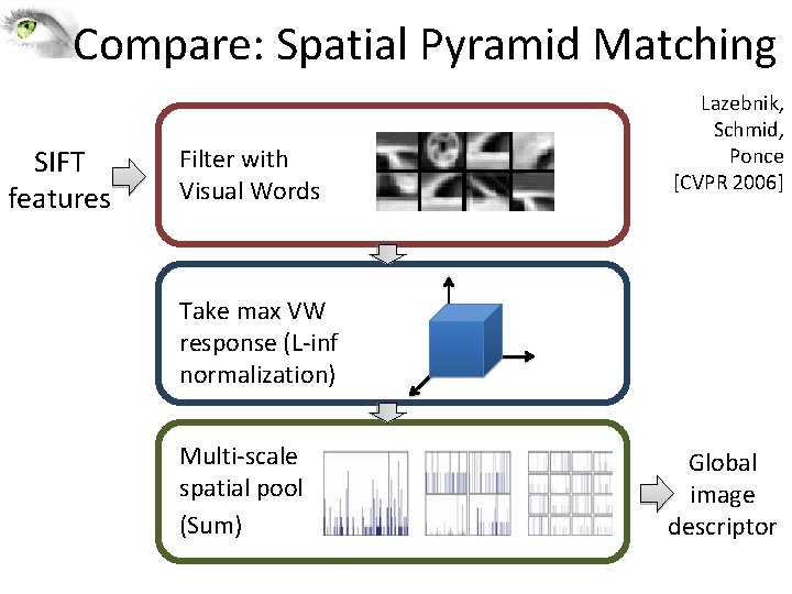
Compare: Spatial Pyramid Matching SIFT features Filter with Visual Words Lazebnik, Schmid, Ponce [CVPR 2006] Take max VW response (L-inf normalization) Multi-scale spatial pool (Sum) Global image descriptor

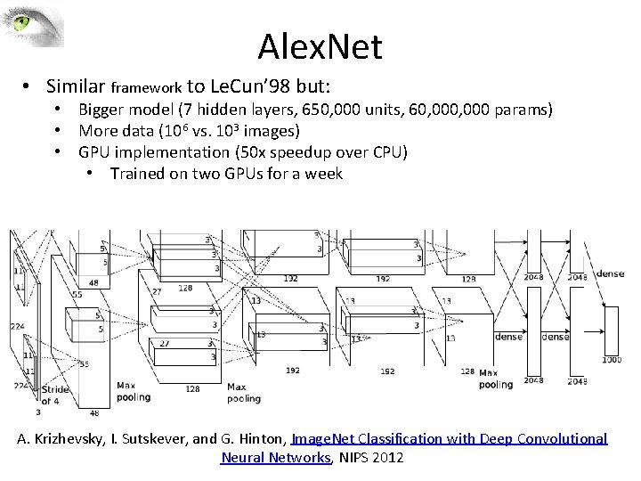
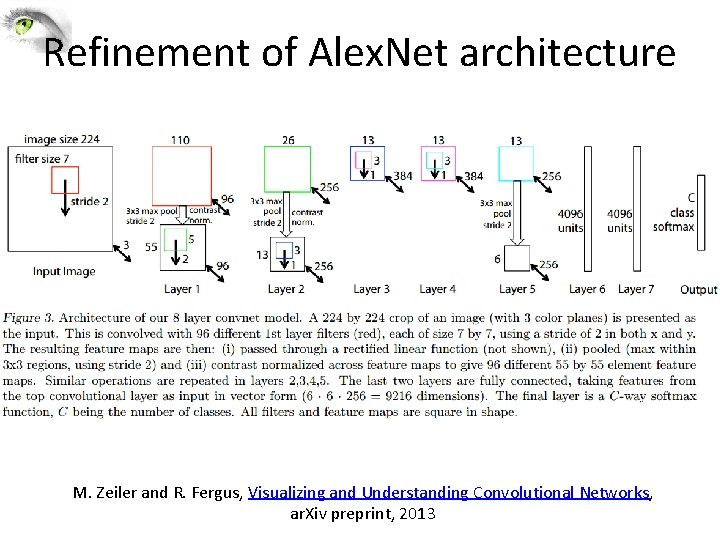
Alex. Net • Similar framework to Le. Cun’ 98 but: • Bigger model (7 hidden layers, 650, 000 units, 60, 000 params) • More data (106 vs. 103 images) • GPU implementation (50 x speedup over CPU) • Trained on two GPUs for a week A. Krizhevsky, I. Sutskever, and G. Hinton, Image. Net Classification with Deep Convolutional Neural Networks, NIPS 2012

Refinement of Alex. Net architecture M. Zeiler and R. Fergus, Visualizing and Understanding Convolutional Networks, ar. Xiv preprint, 2013

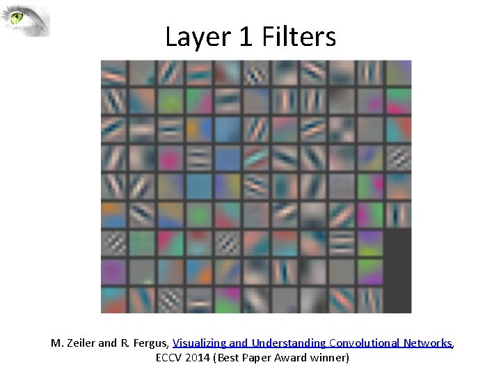
Layer 1 Filters M. Zeiler and R. Fergus, Visualizing and Understanding Convolutional Networks, ECCV 2014 (Best Paper Award winner)

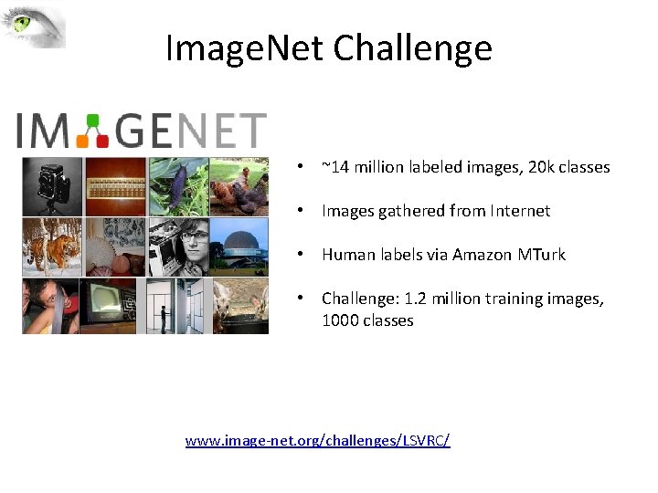
Image. Net Challenge • ~14 million labeled images, 20 k classes • Images gathered from Internet • Human labels via Amazon MTurk • Challenge: 1. 2 million training images, 1000 classes www. image-net. org/challenges/LSVRC/

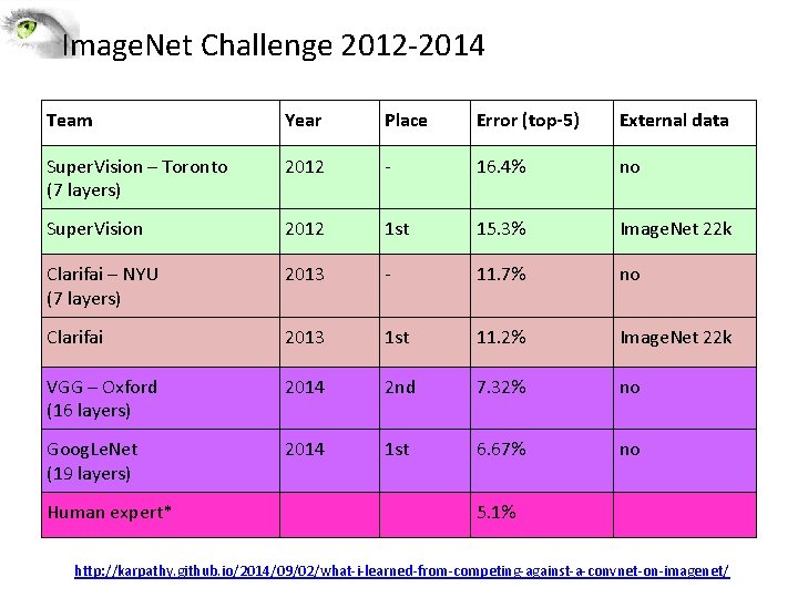
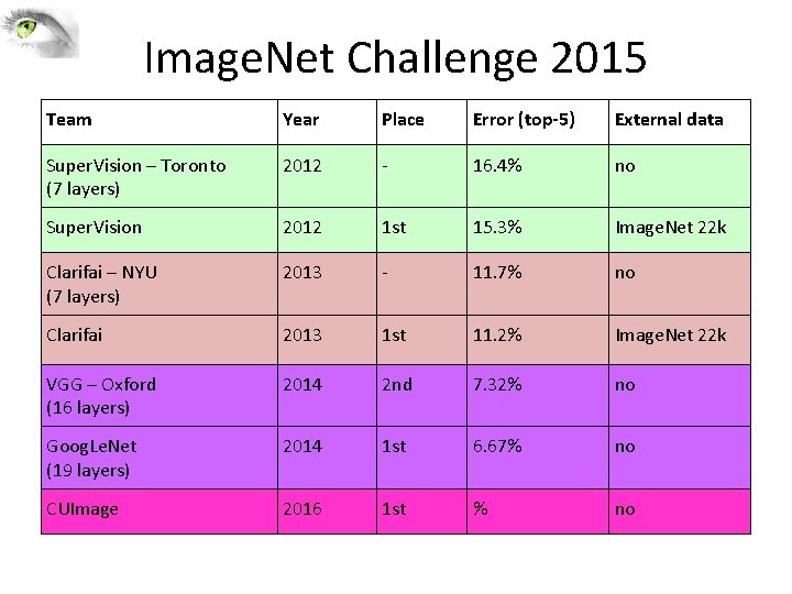
Image. Net Challenge 2012 -2014 Team Year Place Error (top-5) External data Super. Vision – Toronto (7 layers) 2012 - 16. 4% no Super. Vision 2012 1 st 15. 3% Image. Net 22 k Clarifai – NYU (7 layers) 2013 - 11. 7% no Clarifai 2013 1 st 11. 2% Image. Net 22 k VGG – Oxford (16 layers) 2014 2 nd 7. 32% no Goog. Le. Net (19 layers) 2014 1 st 6. 67% no Human expert* 5. 1% http: //karpathy. github. io/2014/09/02/what-i-learned-from-competing-against-a-convnet-on-imagenet/

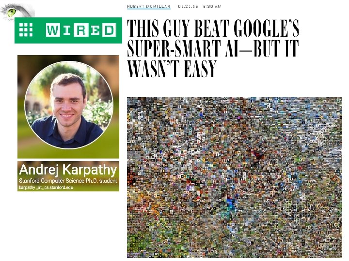
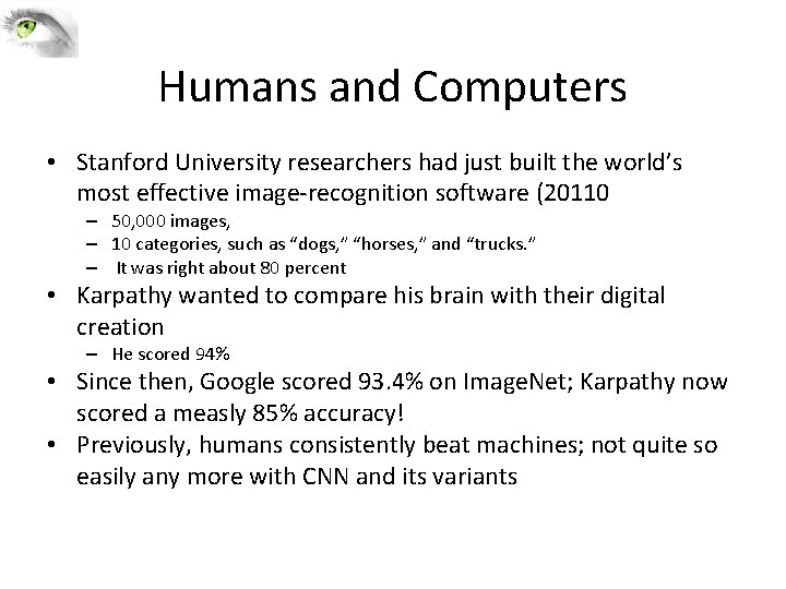
Humans and Computers • Stanford University researchers had just built the world’s most effective image-recognition software (20110 – 50, 000 images, – 10 categories, such as “dogs, ” “horses, ” and “trucks. ” – It was right about 80 percent • Karpathy wanted to compare his brain with their digital creation – He scored 94% • Since then, Google scored 93. 4% on Image. Net; Karpathy now scored a measly 85% accuracy! • Previously, humans consistently beat machines; not quite so easily any more with CNN and its variants

Image. Net Challenge 2015 Team Year Place Error (top-5) External data Super. Vision – Toronto (7 layers) 2012 - 16. 4% no Super. Vision 2012 1 st 15. 3% Image. Net 22 k Clarifai – NYU (7 layers) 2013 - 11. 7% no Clarifai 2013 1 st 11. 2% Image. Net 22 k VGG – Oxford (16 layers) 2014 2 nd 7. 32% no Goog. Le. Net (19 layers) 2014 1 st 6. 67% no CUImage 2016 1 st % no

• • • Deep learning packages Caffe Torch Theano Tensor. Flow Matconvnet … http: //deeplearning. net/software_links/

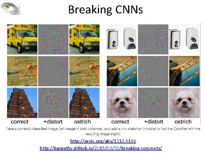
Breaking CNNs http: //arxiv. org/abs/1312. 6199 http: //karpathy. github. io/2015/03/30/breaking-convnets/

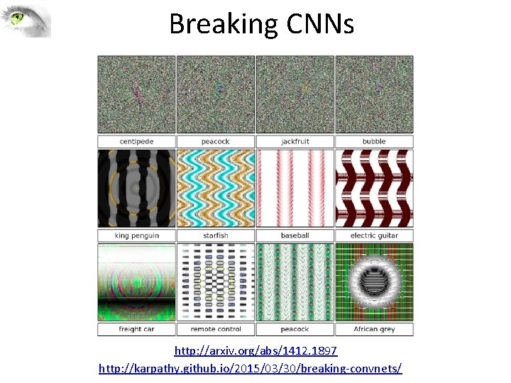
Breaking CNNs http: //arxiv. org/abs/1412. 1897 http: //karpathy. github. io/2015/03/30/breaking-convnets/

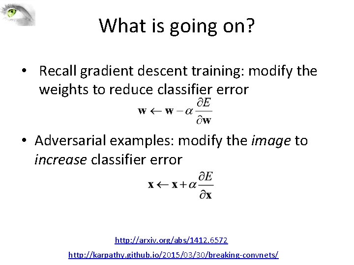
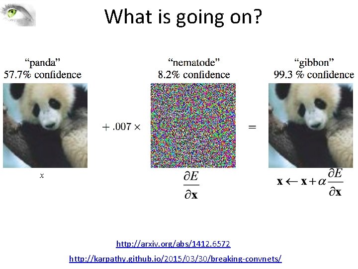
What is going on? • Recall gradient descent training: modify the weights to reduce classifier error • Adversarial examples: modify the image to increase classifier error http: //arxiv. org/abs/1412. 6572 http: //karpathy. github. io/2015/03/30/breaking-convnets/

What is going on? x http: //arxiv. org/abs/1412. 6572 http: //karpathy. github. io/2015/03/30/breaking-convnets/

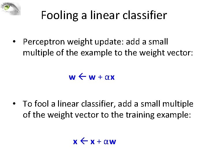
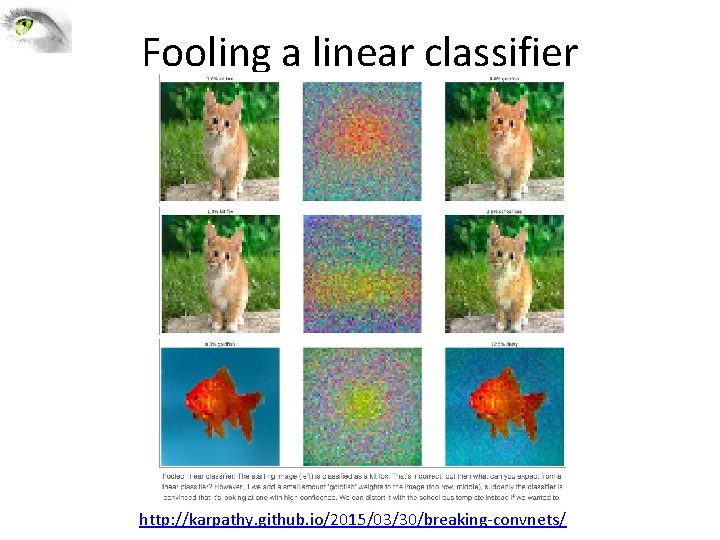
Fooling a linear classifier • Perceptron weight update: add a small multiple of the example to the weight vector: w w + αx • To fool a linear classifier, add a small multiple of the weight vector to the training example: x x + αw

Fooling a linear classifier http: //karpathy. github. io/2015/03/30/breaking-convnets/

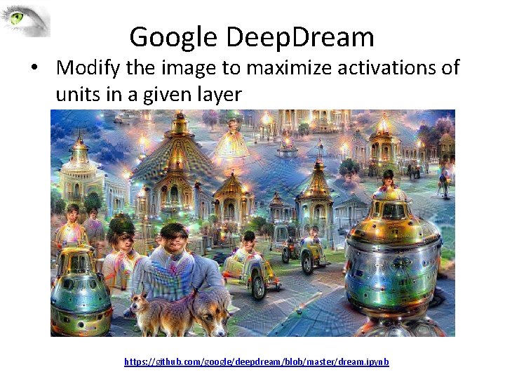
Google Deep. Dream • Modify the image to maximize activations of units in a given layer https: //github. com/google/deepdream/blob/master/dream. ipynb

Next class • Deep aand conv neural networks – hands on • Readings for next lecture: – Tensor flow tutorial online • Readings for today: – Online deep learning tutorial from Stanford http: //cs 231 n. github. io/convolutional-networks/ 39

Questions 40