CSCI 3333 Data Structures Algorithm Analysis by Dr

CSCI 3333 Data Structures Algorithm Analysis by Dr. Bun Yue Professor of Computer Science yue@uhcl. edu http: //sce. uhcl. edu/yue/ 2013

Acknowledgement Mr. Charles Moen ¡ Dr. Wei Ding ¡ Ms. Krishani Abeysekera ¡ Dr. Michael Goodrich ¡

Algorithm ¡ “A finite set of instructions that specify a sequence of operations to be carried out in order to solve a specific problem or class of problems. ”

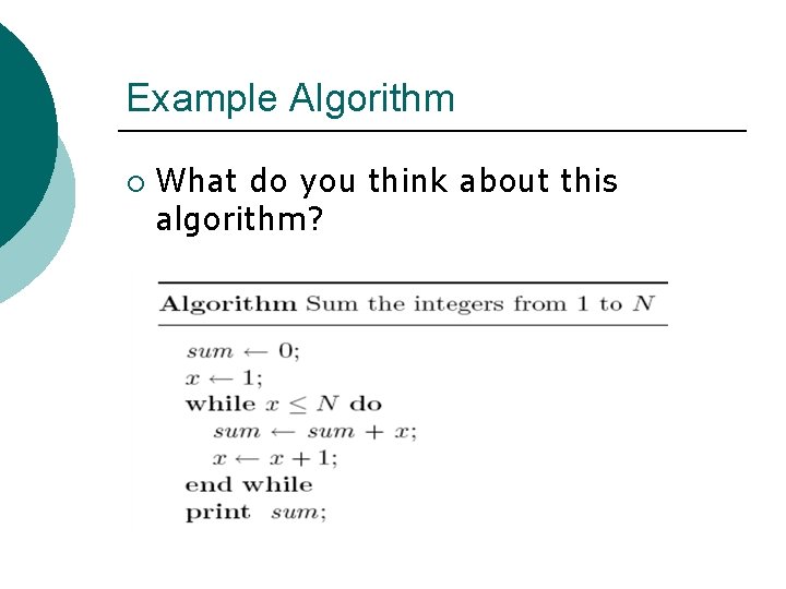
Example Algorithm ¡ What do you think about this algorithm?

Some Properties of Algorithms ¡ A deterministic sequential algorithm should be: l l l Finiteness: Algorithm must complete after a finite number of instructions. Absence of ambiguity: Each step must be clearly defined, having only one interpretation. Definition of sequence: Each step must have a unique defined preceding & succeeding step. The first step (start step) & last step (halt step) must be clearly noted. Input/output: There must be a specified number of input values and result values. Feasibility: It must be possible to perform each instruction.

Specifying Algorithms ¡ There are no universal formal. l l l By English. By Pesudocode By a programming language (not usually desirable. )

Specifying Algorithms ¡ Must be included: l l l ¡ Input: type and meaning Output: type and meaning Instruction sequences. May be included: l l l Assumptions Side effects Pre-conditions and post-conditions

Specifying Algorithms Like sub-programs, algorithms can be broken down into sub-algorithms to reduce complexity. ¡ High level algorithms may use English more. ¡ Low level algorithms may use pseudocode more. ¡

Pseudocode High-level description of an algorithm ¡ More structured than English prose ¡ Less detailed than a program ¡ Preferred notation for describing algorithms ¡ Hide program design issues ¡

Example: Array. Max Algorithm array. Max(A, n) Input array A of n integers Output maximum element value of A current. Max A[0] for i 1 to n 1 do if A[i] current. Max then current. Max A[i] return current. Max ¡ What do you think?

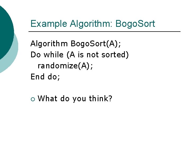
Example Algorithm: Bogo. Sort Algorithm Bogo. Sort(A); Do while (A is not sorted) randomize(A); End do; ¡ What do you think?

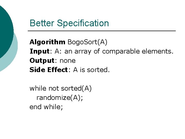
Better Specification Algorithm Bogo. Sort(A) Input: A: an array of comparable elements. Output: none Side Effect: A is sorted. while not sorted(A) randomize(A); end while;

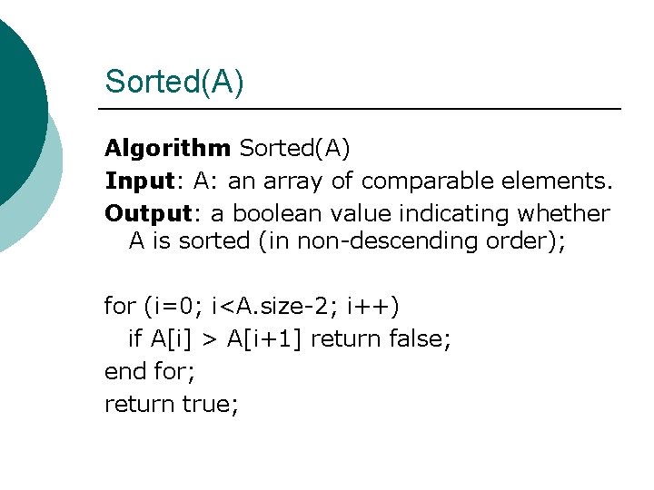
Sorted(A) Algorithm Sorted(A) Input: A: an array of comparable elements. Output: a boolean value indicating whether A is sorted (in non-descending order); for (i=0; i<A. size-2; i++) if A[i] > A[i+1] return false; end for; return true;

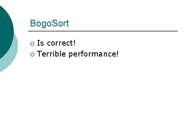
Bogo. Sort Is correct! ¡ Terrible performance! ¡

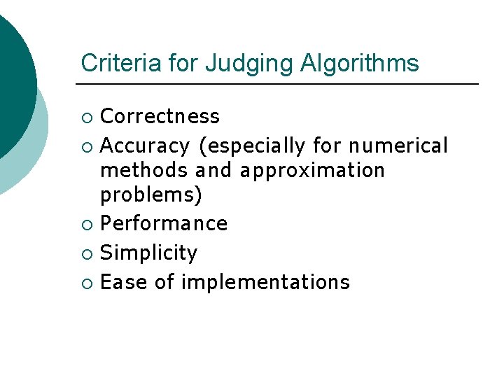
Criteria for Judging Algorithms Correctness ¡ Accuracy (especially for numerical methods and approximation problems) ¡ Performance ¡ Simplicity ¡ Ease of implementations ¡

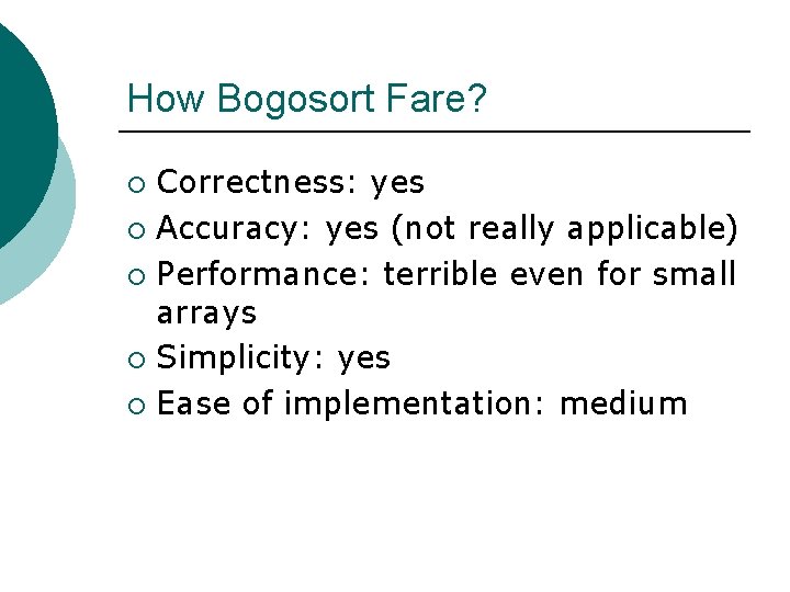
How Bogosort Fare? Correctness: yes ¡ Accuracy: yes (not really applicable) ¡ Performance: terrible even for small arrays ¡ Simplicity: yes ¡ Ease of implementation: medium ¡

Summation Algorithm Correctness: ok. ¡ Performance: bad, proportional to N. ¡ Simplicity: not too bad ¡ Ease: not too bad ¡

Summation Algorithm ¡ A better summation algorithm Algorithm Summation(N) Input: N: Natural Number Output: Summation of 1 to N. return N * (N+1) / 2; ¡ Performance: constant time independent of N.

Performance of Algorithms ¡ Performance of algorithms can be measured by runtime experiments, called benchmark analysis.

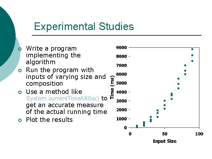
Experimental Studies ¡ ¡ Write a program implementing the algorithm Run the program with inputs of varying size and composition Use a method like System. current. Time. Millis() to get an accurate measure of the actual running time Plot the results

Limitations of Experiments ¡ It is necessary to implement the algorithm, which may: l l be difficult, introduce implementation related performance issues. Results may not be indicative of the running time on other inputs not included in the experiment. ¡ In order to compare two algorithms, the same hardware and software environments must be used. ¡

Theoretical Analysis Uses a high-level description of the algorithm instead of an implementation ¡ Characterizes running time as a function of the input sizes (usually n) ¡ Takes into account all possible inputs ¡ Allows us to evaluate the speed of an algorithm independent of the hardware/software environment ¡

Analysis Tools (Goodrich, 166) Asymptotic Analysis ¡ ¡ ¡ Developed by computer scientists for analyzing the running time of algorithms Describes the running time of an algorithm in terms of the size of the input – in other words, how well does it “scale” as the input gets larger The most common metric used is: l l Upper bound of an algorithm Called the Big-Oh of an algorithm, O(n) 23

Analysis Tools (Goodrich web page) Algorithm Analysis Use asymptotic analysis ¡ Assume that we are using an idealized computer called the Random Access Machine (RAM) ¡ l l ¡ CPU Unlimited amount of memory Accessing a memory cell takes one unit of time Primitive operations take one unit of time Perform the analysis on the pseudocode 24

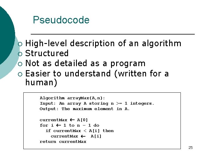
Analysis Tools (Goodrich, 48, 166) Pseudocode High-level description of an algorithm ¡ Structured ¡ Not as detailed as a program ¡ Easier to understand (written for a human) ¡ Algorithm array. Max(A, n): Input: An array A storing n >= 1 integers. Output: The maximum element in A. current. Max A[0] for i 1 to n – 1 do if current. Max < A[i] then current. Max A[i] return current. Max 25

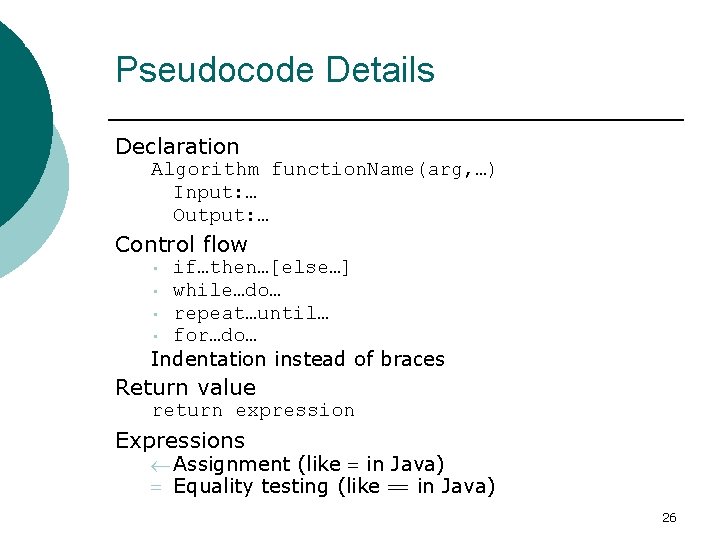
Analysis Tools (Goodrich, 48) Pseudocode Details Declaration Algorithm function. Name(arg, …) Input: … Output: … Control flow if…then…[else…] • while…do… • repeat…until… • for…do… Indentation instead of braces • Return value return expression Expressions Assignment (like in Java) Equality testing (like in Java) 26

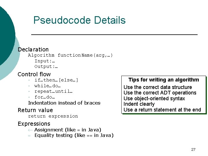
Analysis Tools (Goodrich, 48) Pseudocode Details Declaration Algorithm function. Name(arg, …) Input: … Output: … Control flow if…then…[else…] • while…do… • repeat…until… • for…do… Indentation instead of braces • Return value Tips for writing an algorithm Use the correct data structure Use the correct ADT operations Use object-oriented syntax Indent clearly Use a return statement at the end return expression Expressions Assignment (like in Java) Equality testing (like in Java) 27

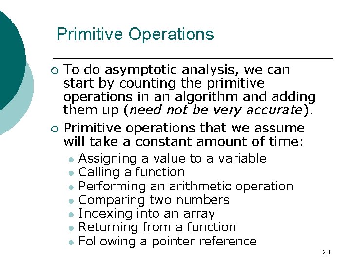
Analysis Tools (Goodrich, 164– 165) Primitive Operations ¡ ¡ To do asymptotic analysis, we can start by counting the primitive operations in an algorithm and adding them up (need not be very accurate). Primitive operations that we assume will take a constant amount of time: l l l l Assigning a value to a variable Calling a function Performing an arithmetic operation Comparing two numbers Indexing into an array Returning from a function Following a pointer reference 28

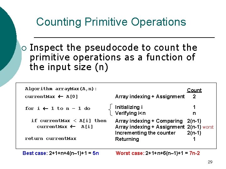
Analysis Tools (Goodrich, 166) Counting Primitive Operations ¡ Inspect the pseudocode to count the primitive operations as a function of the input size (n) Algorithm array. Max(A, n): current. Max A[0] for i 1 to n – 1 do if current. Max < A[i] then current. Max A[i] return current. Max Best case: 2+1+n+4(n– 1)+1 = 5 n Count Array indexing + Assignment 2 Initializing i Verifying i<n 1 n Array indexing + Comparing 2(n-1) Array indexing + Assignment 2(n-1) worst Incrementing the counter 2(n-1) Returning 1 Worst case: 2+1+n+6(n– 1)+1 = 7 n-2 29

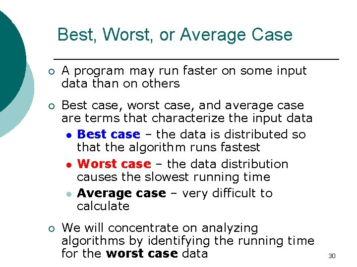
Analysis Tools (Goodrich, 165) Best, Worst, or Average Case ¡ A program may run faster on some input data than on others ¡ Best case, worst case, and average case are terms that characterize the input data l Best case – the data is distributed so that the algorithm runs fastest l Worst case – the data distribution causes the slowest running time l Average case – very difficult to calculate ¡ We will concentrate on analyzing algorithms by identifying the running time for the worst case data 30

Analysis Tools (Goodrich, 166) Running Time of array. Max ¡ Worst case running time of array. Max f(n) = (7 n – 2) primitive operations ¡ Actual running time depends on the speed of the primitive operations—some of them are faster than others l Let t = speed of the slowest primitive operation l Let f(n) = the worst-case running time of array. Max f(n) = t (7 n – 2) 31

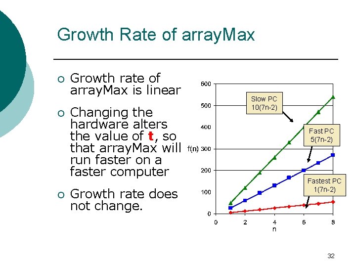
Analysis Tools (Goodrich, 166) Growth Rate of array. Max ¡ ¡ ¡ Growth rate of array. Max is linear Changing the hardware alters the value of t, so that array. Max will run faster on a faster computer Growth rate does not change. Slow PC 10(7 n-2) Fast PC 5(7 n-2) Fastest PC 1(7 n-2) 32

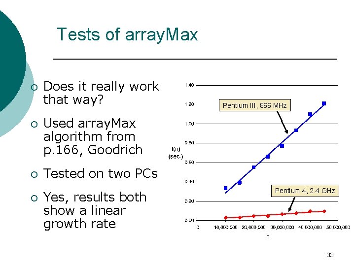
Analysis Tools Tests of array. Max ¡ Does it really work that way? ¡ Used array. Max algorithm from p. 166, Goodrich ¡ Tested on two PCs ¡ Yes, results both show a linear growth rate Pentium III, 866 MHz Pentium 4, 2. 4 GHz 33

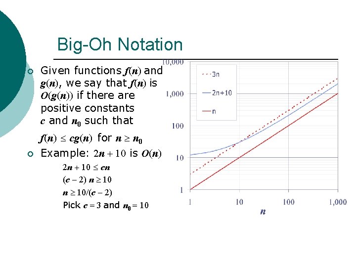
Big-Oh Notation ¡ ¡ Given functions f(n) and g(n), we say that f(n) is O(g(n)) if there are positive constants c and n 0 such that f(n) cg(n) for n n 0 Example: 2 n + 10 is O(n) 2 n + 10 cn (c 2) n 10/(c 2) Pick c 3 and n 0 10

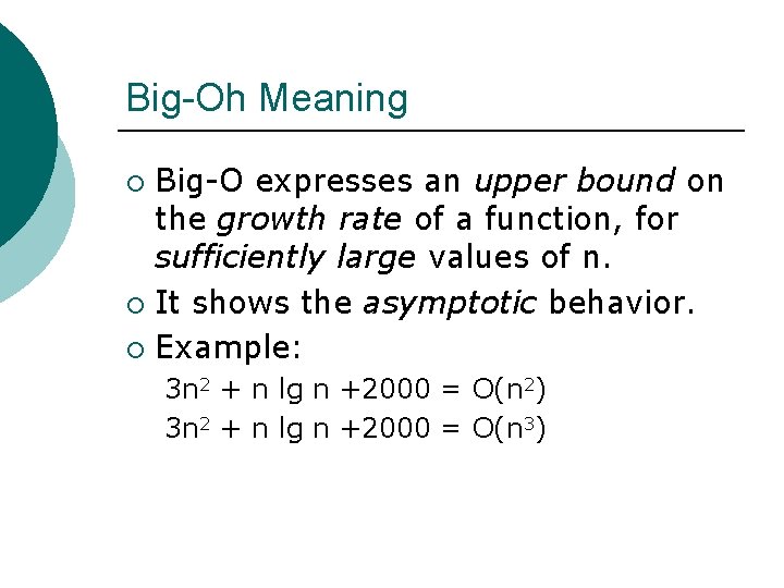
Big-Oh Meaning Big-O expresses an upper bound on the growth rate of a function, for sufficiently large values of n. ¡ It shows the asymptotic behavior. ¡ Example: ¡ 3 n 2 + n lg n +2000 = O(n 2) 3 n 2 + n lg n +2000 = O(n 3)

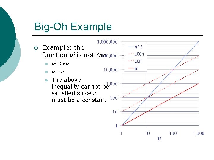
Big-Oh Example ¡ Example: the function n 2 is not O(n) l l l n 2 cn n c The above inequality cannot be satisfied since c must be a constant

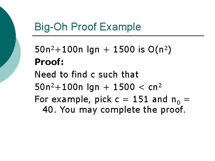
Big-Oh Proof Example 50 n 2+100 n lgn + 1500 is O(n 2) Proof: Need to find c such that 50 n 2+100 n lgn + 1500 < cn 2 For example, pick c = 151 and n 0 = 40. You may complete the proof.

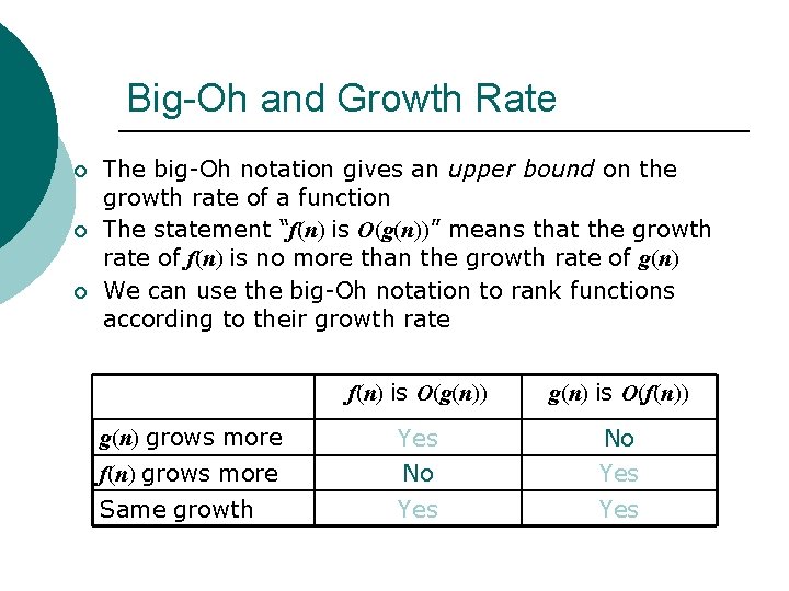
Big-Oh and Growth Rate ¡ ¡ ¡ The big-Oh notation gives an upper bound on the growth rate of a function The statement “f(n) is O(g(n))” means that the growth rate of f(n) is no more than the growth rate of g(n) We can use the big-Oh notation to rank functions according to their growth rate f(n) is O(g(n)) g(n) is O(f(n)) g(n) grows more Yes No f(n) grows more No Yes Same growth Yes

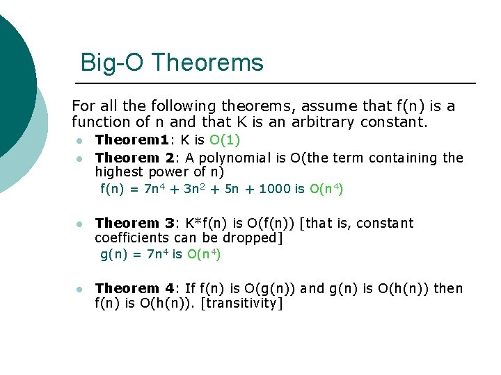
Big-O Theorems For all the following theorems, assume that f(n) is a function of n and that K is an arbitrary constant. l l Theorem 1: K is O(1) Theorem 2: A polynomial is O(the term containing the highest power of n) f(n) = 7 n 4 + 3 n 2 + 5 n + 1000 is O(n 4) l Theorem 3: K*f(n) is O(f(n)) [that is, constant coefficients can be dropped] g(n) = 7 n 4 is O(n 4) l Theorem 4: If f(n) is O(g(n)) and g(n) is O(h(n)) then f(n) is O(h(n)). [transitivity]

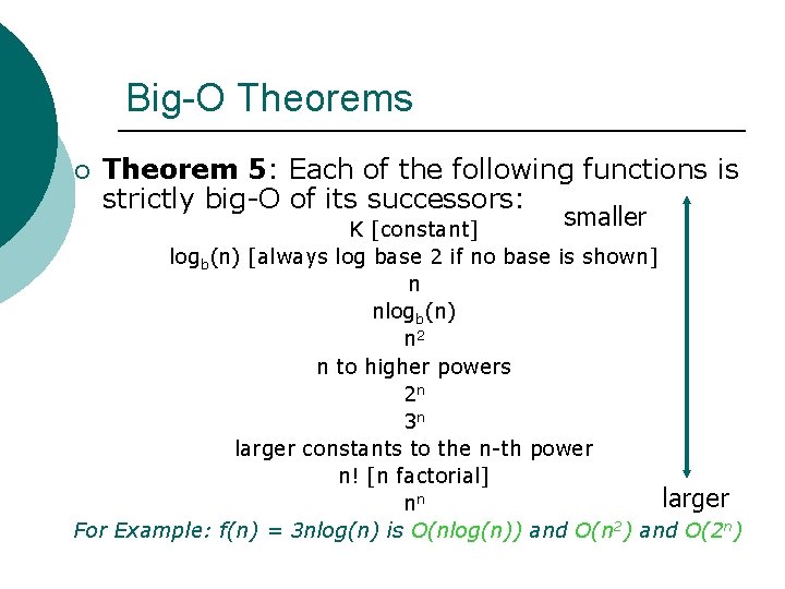
Big-O Theorems ¡ Theorem 5: Each of the following functions is strictly big-O of its successors: smaller K [constant] logb(n) [always log base 2 if no base is shown] n nlogb(n) n 2 n to higher powers 2 n 3 n larger constants to the n-th power n! [n factorial] larger nn For Example: f(n) = 3 nlog(n) is O(nlog(n)) and O(n 2) and O(2 n)

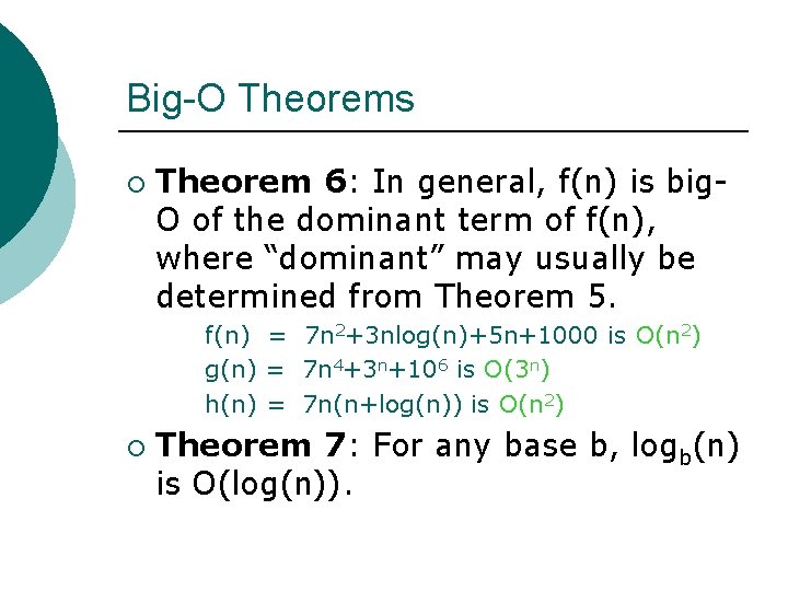
Big-O Theorems ¡ Theorem 6: In general, f(n) is big. O of the dominant term of f(n), where “dominant” may usually be determined from Theorem 5. f(n) = 7 n 2+3 nlog(n)+5 n+1000 is O(n 2) g(n) = 7 n 4+3 n+106 is O(3 n) h(n) = 7 n(n+log(n)) is O(n 2) ¡ Theorem 7: For any base b, logb(n) is O(log(n)).

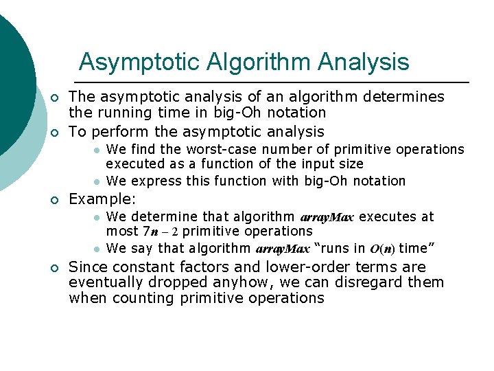
Asymptotic Algorithm Analysis ¡ ¡ The asymptotic analysis of an algorithm determines the running time in big-Oh notation To perform the asymptotic analysis l l ¡ Example: l l ¡ We find the worst-case number of primitive operations executed as a function of the input size We express this function with big-Oh notation We determine that algorithm array. Max executes at most 7 n 2 primitive operations We say that algorithm array. Max “runs in O(n) time” Since constant factors and lower-order terms are eventually dropped anyhow, we can disregard them when counting primitive operations

Example: Computing Prefix Averages We further illustrate asymptotic analysis with two algorithms for prefix averages ¡ The i-th prefix average of an array X is average of the first (i + 1) elements of X: A[i] (X[0] + X[1] + … + X[i])/(i+1) ¡ ¡ Computing the array A of prefix averages of another array X has applications to financial analysis

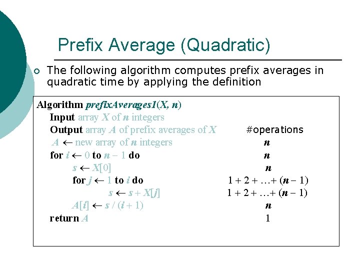
Prefix Average (Quadratic) ¡ The following algorithm computes prefix averages in quadratic time by applying the definition Algorithm prefix. Averages 1(X, n) Input array X of n integers Output array A of prefix averages of X A new array of n integers for i 0 to n 1 do s X[0] for j 1 to i do s s + X[j] A[i] s / (i + 1) return A #operations n n n 1 + 2 + …+ (n 1) n 1

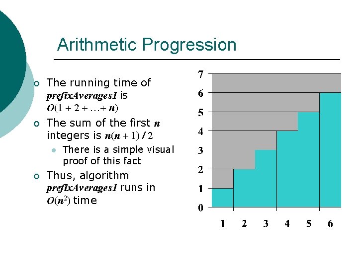
Arithmetic Progression ¡ ¡ The running time of prefix. Averages 1 is O(1 + 2 + …+ n) The sum of the first n integers is n(n + 1) / 2 l ¡ There is a simple visual proof of this fact Thus, algorithm prefix. Averages 1 runs in O(n 2) time

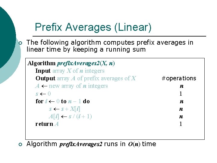
Prefix Averages (Linear) ¡ The following algorithm computes prefix averages in linear time by keeping a running sum Algorithm prefix. Averages 2(X, n) Input array X of n integers Output array A of prefix averages of X A new array of n integers s 0 for i 0 to n 1 do s s + X[i] A[i] s / (i + 1) return A ¡ Algorithm prefix. Averages 2 runs in O(n) time #operations n 1 n n n 1

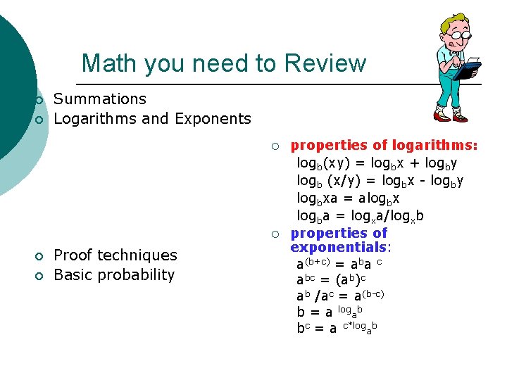
Math you need to Review ¡ ¡ Summations Logarithms and Exponents ¡ ¡ Proof techniques Basic probability properties of logarithms: logb(xy) = logbx + logby logb (x/y) = logbx - logby logbxa = alogbx logba = logxa/logxb properties of exponentials: a(b+c) = aba c abc = (ab)c ab /ac = a(b-c) b = a logab bc = a c*logab

Relatives of Big-Oh ¡ big-Omega (Lower bound) l f(n) is (g(n)) if there is a constant c > 0 and an integer constant n 0 1 such that f(n) c • g(n) for n n 0 ¡ big-Theta (order) l f(n) is (g(n)) if there are constants c’ > 0 and c’’ > 0 and an integer constant n 0 1 such that c’ • g(n) f(n) c’’ • g(n) for n n 0

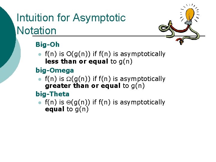
Intuition for Asymptotic Notation Big-Oh l f(n) is O(g(n)) if f(n) is asymptotically less than or equal to g(n) big-Omega l f(n) is (g(n)) if f(n) is asymptotically greater than or equal to g(n) big-Theta l f(n) is (g(n)) if f(n) is asymptotically equal to g(n)

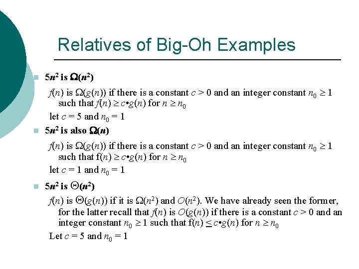
Relatives of Big-Oh Examples n 5 n 2 is (n 2) n f(n) is (g(n)) if there is a constant c > 0 and an integer constant n 0 1 such that f(n) c • g(n) for n n 0 let c = 5 and n 0 = 1 5 n 2 is also (n) f(n) is (g(n)) if there is a constant c > 0 and an integer constant n 0 1 such that f(n) c • g(n) for n n 0 let c = 1 and n 0 = 1 n 5 n 2 is (n 2) f(n) is (g(n)) if it is (n 2) and O(n 2). We have already seen the former, for the latter recall that f(n) is O(g(n)) if there is a constant c > 0 and an integer constant n 0 1 such that f(n) < c • g(n) for n n 0 Let c = 5 and n 0 = 1

Algorithm Complexity analysis (using Big-O) applies to algorithms, not problems. ¡ May be applied to measure: ¡ l l l Best case: not very useful. Worst case: most useful and common. Average case: very useful but can be very difficult: ¡ Depend on the input distribution.

What can be analyzed? ¡ Primitive operations: l l CPU/primary memory I/O Function call Communication Primary memory usage ¡ Secondary memory usage ¡ Number of processor used ¡ … ¡

Questions and Comments?