CSCI 2950 C Lecture 10 Cancer Genomics Duplications

CSCI 2950 -C Lecture 10 Cancer Genomics: Duplications October 21, 2008 http: //cs. brown. edu/courses/csci 2950 -c/

Outline • Cancer Genomes 1. Duplications and End Sequence Profiling 2. Comparative Genomic Hybridization • Cancer Progression Models

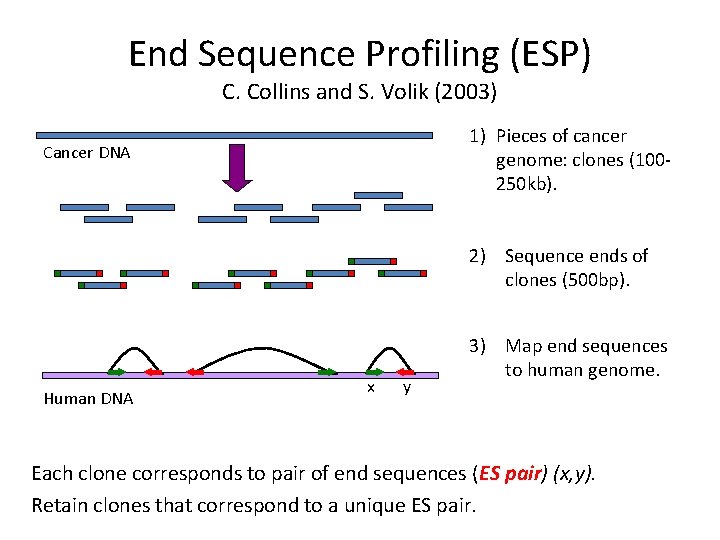
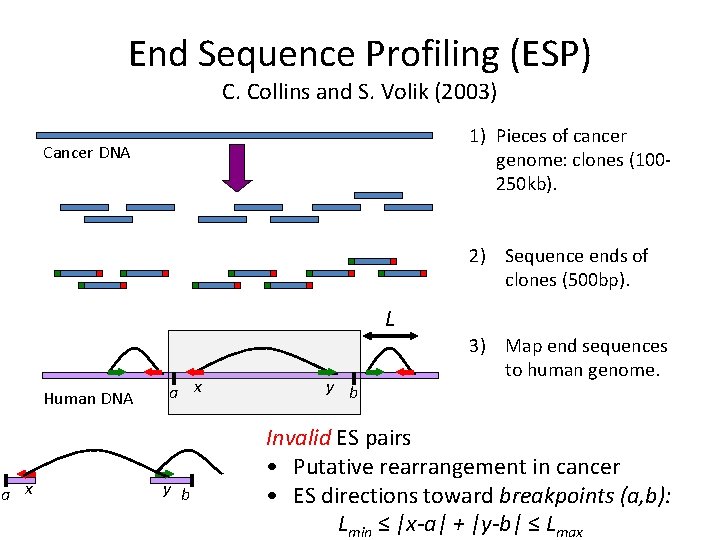
End Sequence Profiling (ESP) C. Collins and S. Volik (2003) 1) Pieces of cancer genome: clones (100250 kb). Cancer DNA 2) Sequence ends of clones (500 bp). Human DNA x y 3) Map end sequences to human genome. Each clone corresponds to pair of end sequences (ES pair) (x, y). Retain clones that correspond to a unique ES pair.

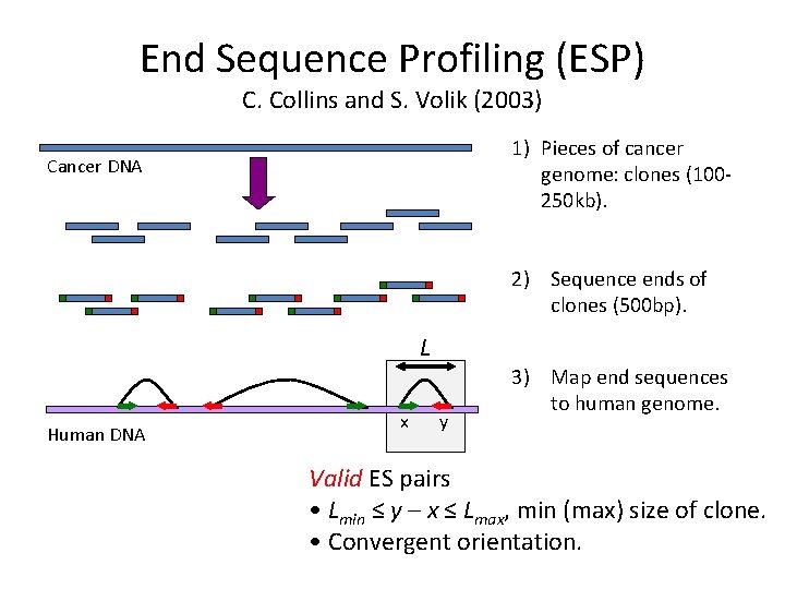
End Sequence Profiling (ESP) C. Collins and S. Volik (2003) 1) Pieces of cancer genome: clones (100250 kb). Cancer DNA 2) Sequence ends of clones (500 bp). L Human DNA x y 3) Map end sequences to human genome. Valid ES pairs • Lmin ≤ y – x ≤ Lmax, min (max) size of clone. • Convergent orientation.

End Sequence Profiling (ESP) C. Collins and S. Volik (2003) 1) Pieces of cancer genome: clones (100250 kb). Cancer DNA 2) Sequence ends of clones (500 bp). L Human DNA a x y b 3) Map end sequences to human genome. Invalid ES pairs • Putative rearrangement in cancer • ES directions toward breakpoints (a, b): Lmin ≤ |x-a| + |y-b| ≤ Lmax

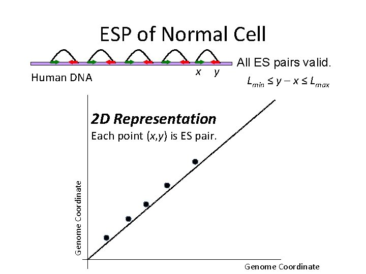
ESP of Normal Cell Human DNA x y All ES pairs valid. Lmin ≤ y – x ≤ Lmax 2 D Representation Genome Coordinate Each point (x, y) is ES pair. Genome Coordinate

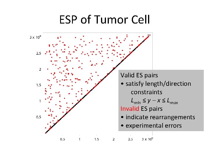
ESP of Tumor Cell Valid ES pairs • satisfy length/direction constraints Lmin ≤ y – x ≤ Lmax Invalid ES pairs • indicate rearrangements • experimental errors

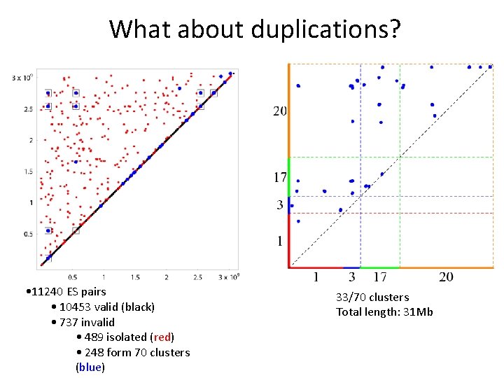
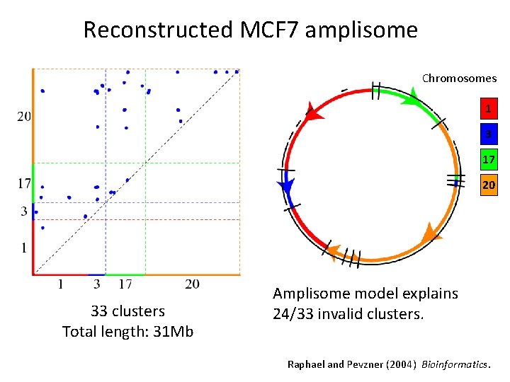
What about duplications? • 11240 ES pairs • 10453 valid (black) • 737 invalid • 489 isolated (red) • 248 form 70 clusters (blue) 33/70 clusters Total length: 31 Mb

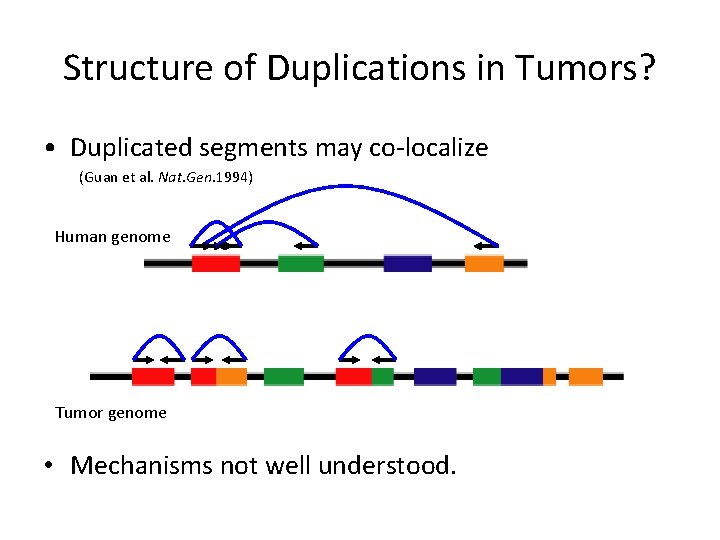
Structure of Duplications in Tumors? • Duplicated segments may co-localize (Guan et al. Nat. Gen. 1994) Human genome Tumor genome • Mechanisms not well understood.

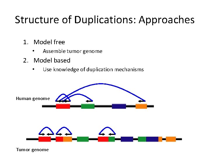
Structure of Duplications: Approaches 1. Model free • Assemble tumor genome 2. Model based • Use knowledge of duplication mechanisms Human genome Tumor genome

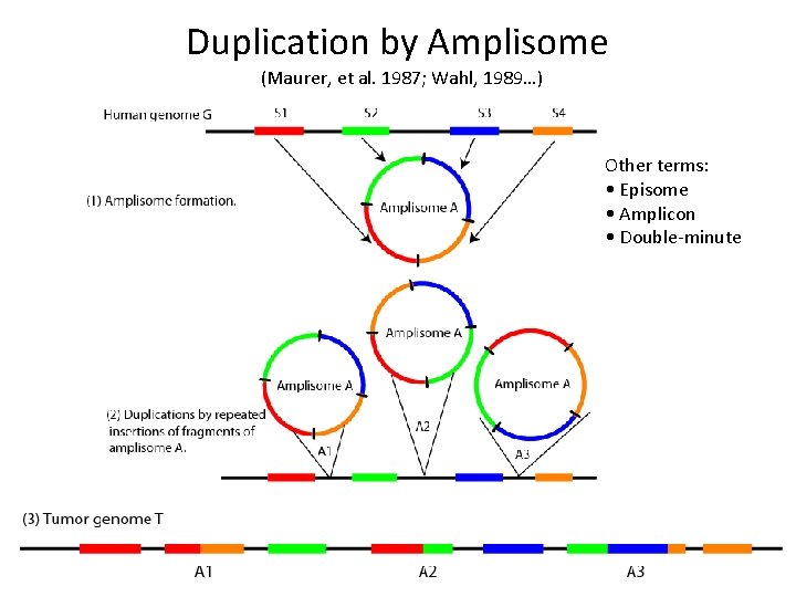
Duplication by Amplisome (Maurer, et al. 1987; Wahl, 1989…) Other terms: • Episome • Amplicon • Double-minute

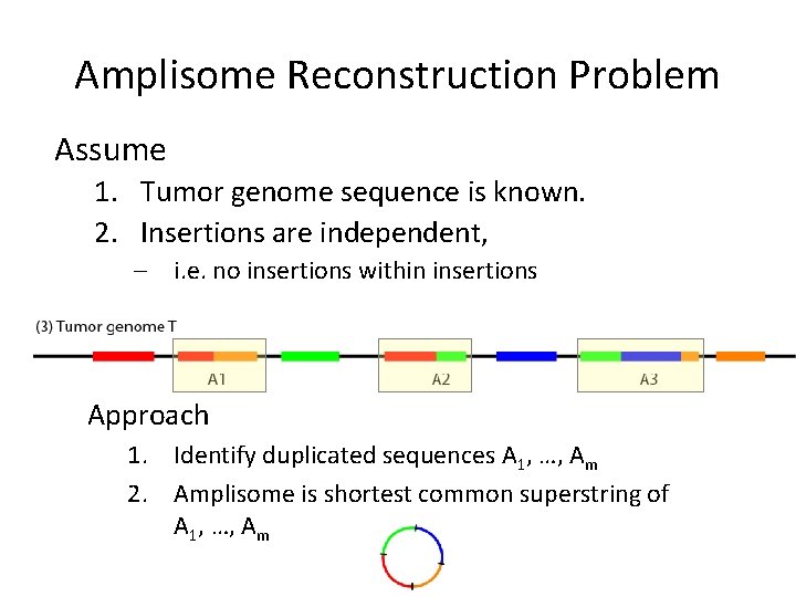
Amplisome Reconstruction Problem Assume 1. Tumor genome sequence is known. 2. Insertions are independent, – i. e. no insertions within insertions Approach 1. Identify duplicated sequences A 1, …, Am 2. Amplisome is shortest common superstring of A 1, …, Am

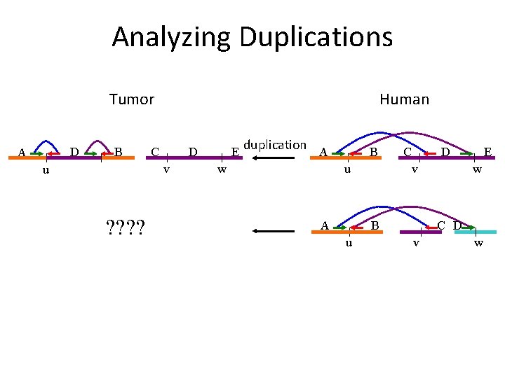
Analyzing Duplications Tumor D A B Human C D v u ? ? E duplication A w B D v u A C B u E w C D v w

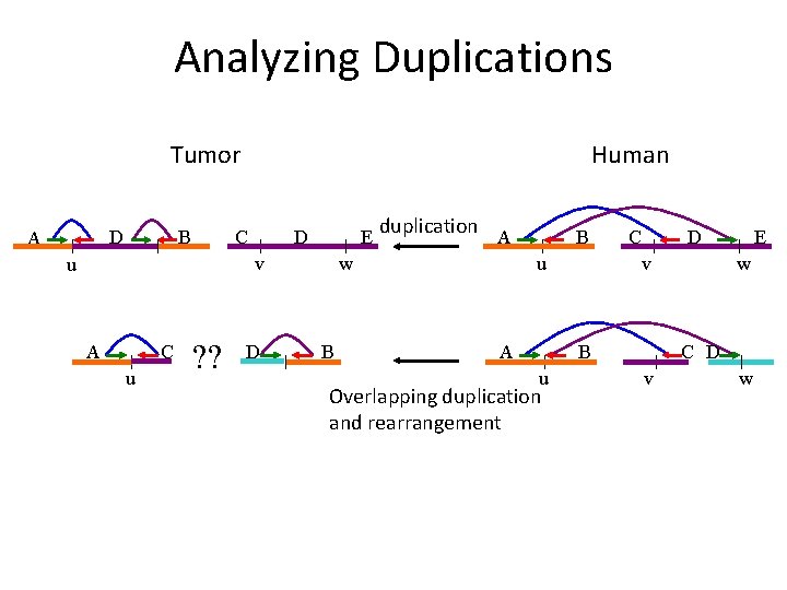
Analyzing Duplications Tumor D A B Human C D E v u A C u ? ? D duplication A w B B D v u A C B u Overlapping duplication and rearrangement E w C D v w

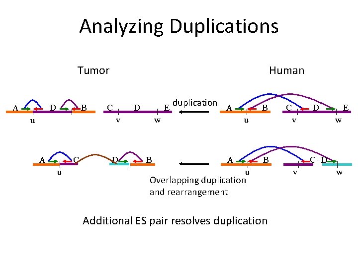
Analyzing Duplications Tumor D A B Human C D E v u A C u D duplication A w B B D v u A C B u Overlapping duplication and rearrangement Additional ES pair resolves duplication E w C D v w

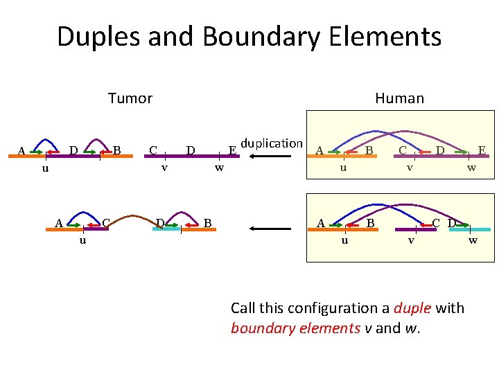
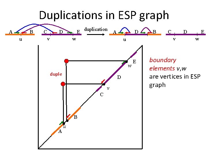
Duples and Boundary Elements Tumor D A B Human C D E v u A C u D duplication A w B B D v u A C B u E w C D v Call this configuration a duple with boundary elements v and w. w

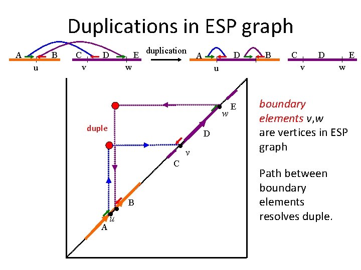
Duplications in ESP graph A B u C E duplication D v D A w w D v C B A u C D v u duple B E E w boundary elements v, w are vertices in ESP graph

Duplications in ESP graph A B u C E duplication D v D A w w D v C B A u C D v u duple B E E w boundary elements v, w are vertices in ESP graph Path between boundary elements resolves duple.

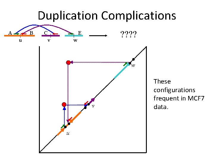
Duplication Complications A B u C ? ? E v w w v u These configurations frequent in MCF 7 data.

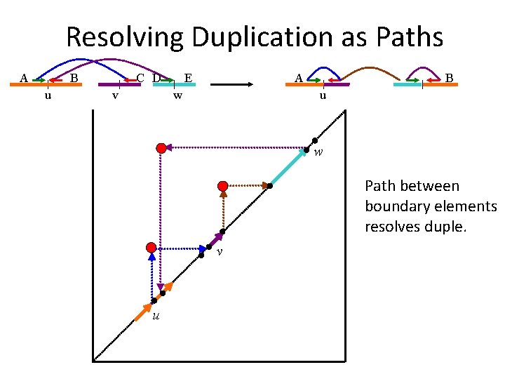
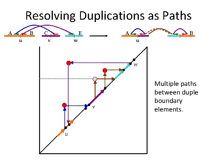
Resolving Duplication as Paths A B u C D v E A w B u w Path between boundary elements resolves duple. v u

Resolving Duplications as Paths A B u C E v A w B u w v u Multiple paths between duple boundary elements.

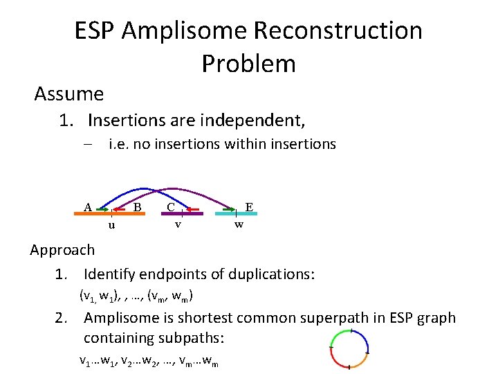
ESP Amplisome Reconstruction Problem Assume 1. Insertions are independent, – i. e. no insertions within insertions A B u C E v w Approach 1. Identify endpoints of duplications: (v 1, w 1), , …, (vm, wm) 2. Amplisome is shortest common superpath in ESP graph containing subpaths: v 1…w 1, v 2…w 2, …, vm…wm

Reconstructed MCF 7 amplisome Chromosomes 1 3 17 20 33 clusters Total length: 31 Mb Amplisome model explains 24/33 invalid clusters. Raphael and Pevzner (2004) Bioinformatics.

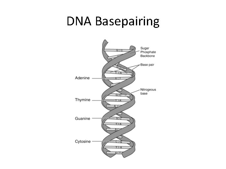
DNA Basepairing

DNA Microarrays

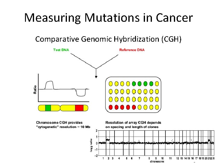
Measuring Mutations in Cancer Comparative Genomic Hybridization (CGH)

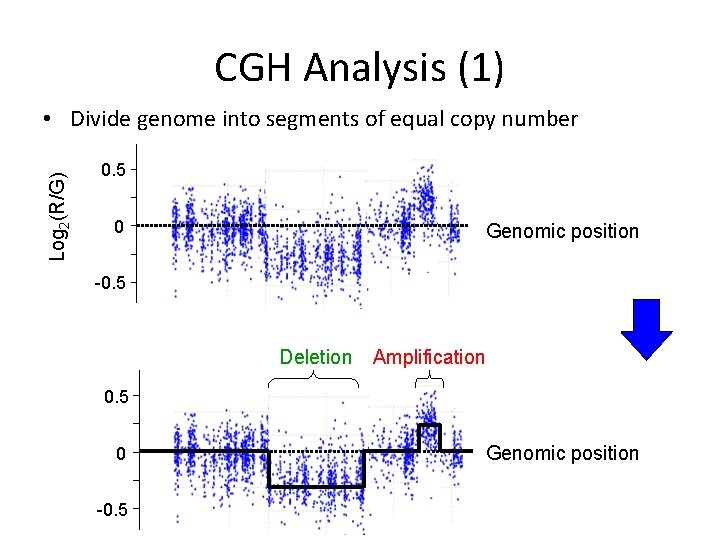
CGH Analysis (1) Log 2(R/G) • Divide genome into segments of equal copy number 0. 5 0 Genomic position -0. 5 Deletion Amplification 0. 5 0 -0. 5 Genomic position

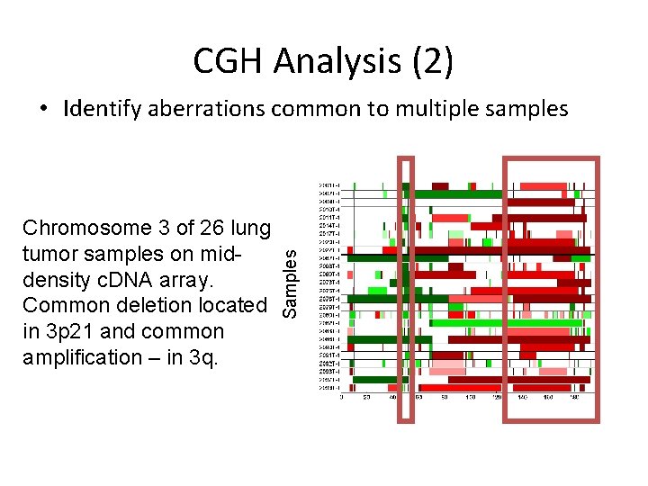
CGH Analysis (2) Chromosome 3 of 26 lung tumor samples on middensity c. DNA array. Common deletion located in 3 p 21 and common amplification – in 3 q. Samples • Identify aberrations common to multiple samples

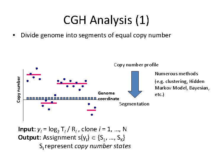
CGH Analysis (1) • Divide genome into segments of equal copy number Copy number profile Genome coordinate Segmentation Input: yi = log 2 Ti / Ri , clone i = 1, …, N Output: Assignment s(yi) {S 1, …, SK} Si represent copy number states Numerous methods (e. g. clustering, Hidden Markov Model, Bayesian, etc. )

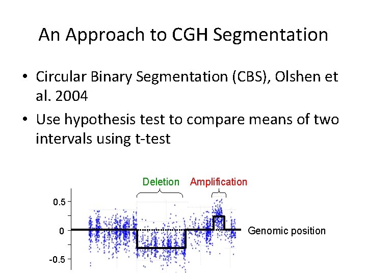
An Approach to CGH Segmentation • Circular Binary Segmentation (CBS), Olshen et al. 2004 • Use hypothesis test to compare means of two intervals using t-test Deletion Amplification 0. 5 0 -0. 5 Genomic position

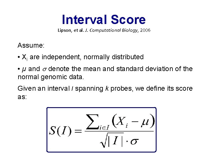
Interval Score Lipson, et al. J. Computational Biology, 2006 Assume: • Xi are independent, normally distributed • µ and denote the mean and standard deviation of the normal genomic data. Given an interval I spanning k probes, we define its score as:

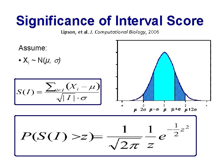
Significance of Interval Score Lipson, et al. J. Computational Biology, 2006 Assume: • Xi ~ N(µ, )

The Max. Interval Problem Input: A vector X=(X 1…Xn) Output: An interval I [1…n], that maximizes S(I ) Other intervals with high scores may be found by recursively calling this function. Exhaustive algorithm: O(n 2)

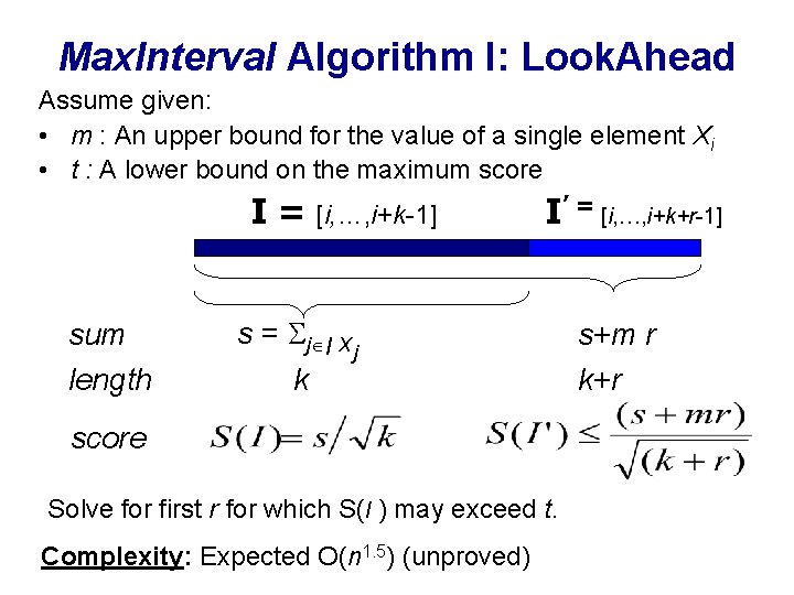
Max. Interval Algorithm I: Look. Ahead Assume given: • m : An upper bound for the value of a single element Xi • t : A lower bound on the maximum score I = [i, …, i+k-1] sum length I’ = [i, …, i+k+r-1] s = j I Xj k score Solve for first r for which S(I ) may exceed t. Complexity: Expected O(n 1. 5) (unproved) s+m r k+r

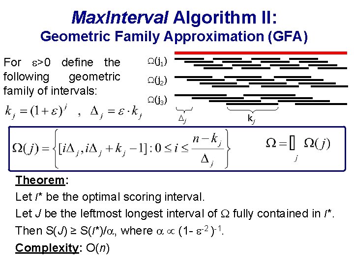
Max. Interval Algorithm II: Geometric Family Approximation (GFA) For >0 define the following geometric family of intervals: (j 1) (j 2) (j 3) j kj Theorem: Let I* be the optimal scoring interval. Let J be the leftmost longest interval of fully contained in I*. Then S(J) ≥ S(I*)/ , where (1 - -2 )-1. Complexity: O(n)

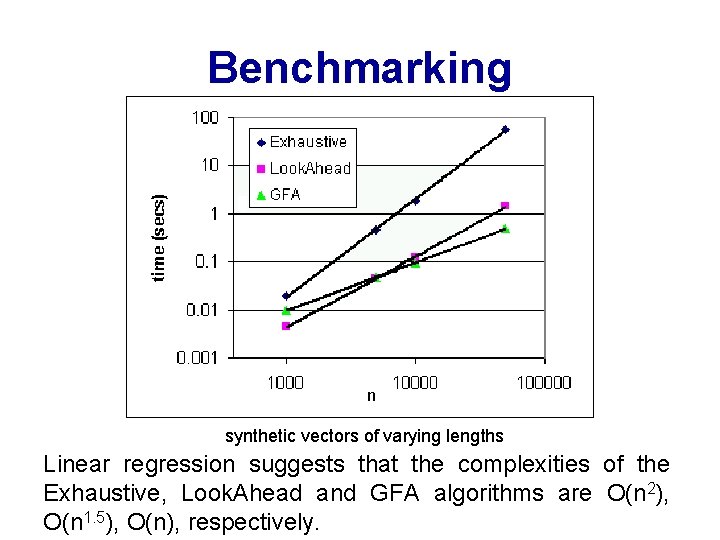
Benchmarking synthetic vectors of varying lengths Linear regression suggests that the complexities of the Exhaustive, Look. Ahead and GFA algorithms are O(n 2), O(n 1. 5), O(n), respectively.

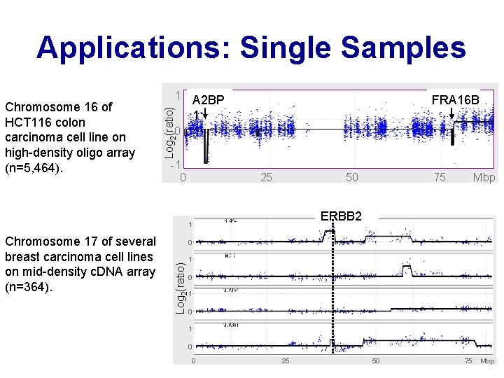
Applications: Single Samples A 2 BP 1 Log 2(ratio) Chromosome 16 of HCT 116 colon carcinoma cell line on high-density oligo array (n=5, 464). 1 FRA 16 B 0 -1 0 25 50 Mbp ERBB 2 1 0 Log 2(ratio) Chromosome 17 of several breast carcinoma cell lines on mid-density c. DNA array (n=364). 75 1 0 1 0 0 25 50 75 Mbp

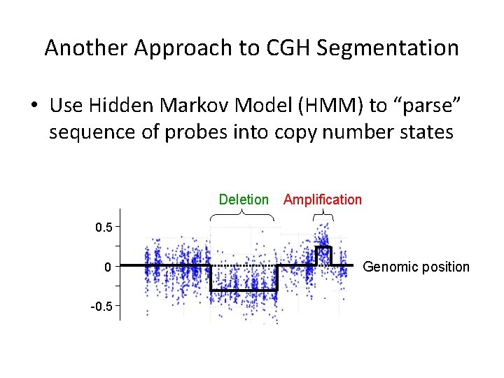
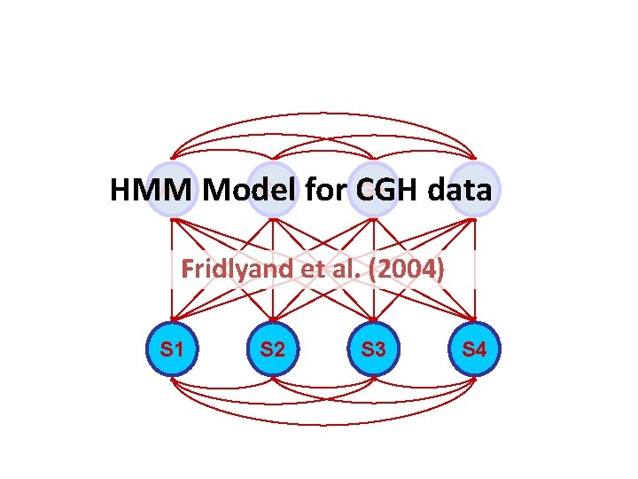
Another Approach to CGH Segmentation • Use Hidden Markov Model (HMM) to “parse” sequence of probes into copy number states Deletion Amplification 0. 5 0 -0. 5 Genomic position

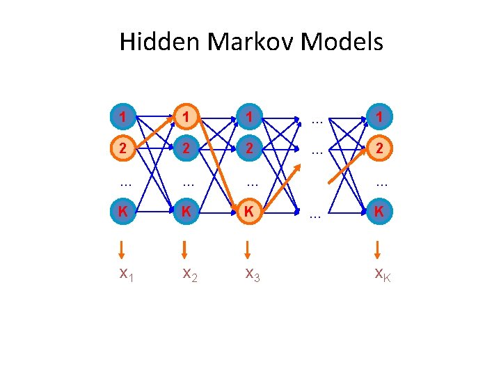
Hidden Markov Models 1 1 1 … 1 2 2 2 … … … K K K x 1 x 2 x 3 … … K x. K

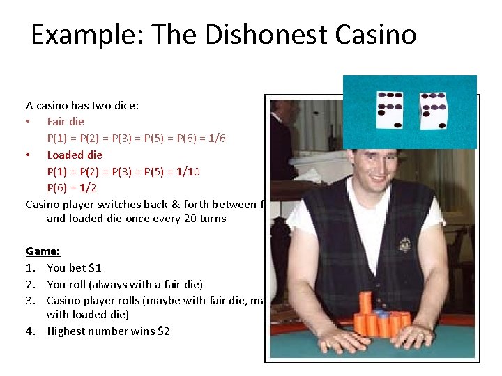
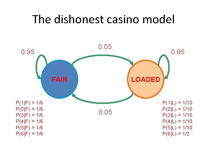
Example: The Dishonest Casino A casino has two dice: • Fair die P(1) = P(2) = P(3) = P(5) = P(6) = 1/6 • Loaded die P(1) = P(2) = P(3) = P(5) = 1/10 P(6) = 1/2 Casino player switches back-&-forth between fair and loaded die once every 20 turns Game: 1. You bet $1 2. You roll (always with a fair die) 3. Casino player rolls (maybe with fair die, maybe with loaded die) 4. Highest number wins $2

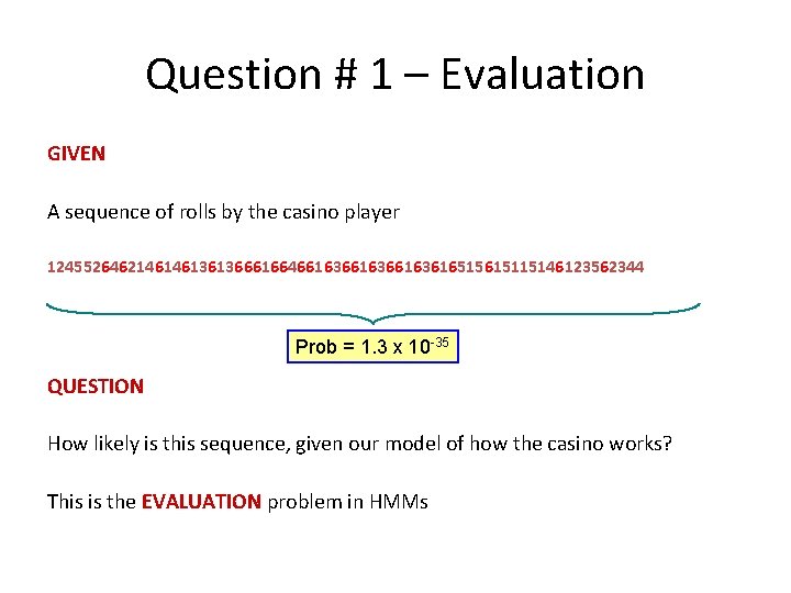
Question # 1 – Evaluation GIVEN A sequence of rolls by the casino player 12455264621461461361366616646616366163616515615115146123562344 Prob = 1. 3 x 10 -35 QUESTION How likely is this sequence, given our model of how the casino works? This is the EVALUATION problem in HMMs

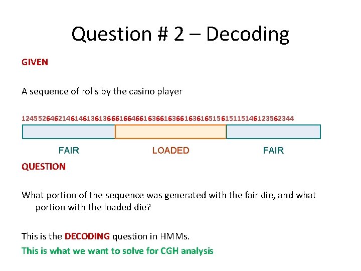
Question # 2 – Decoding GIVEN A sequence of rolls by the casino player 12455264621461461361366616646616366163616515615115146123562344 FAIR LOADED FAIR QUESTION What portion of the sequence was generated with the fair die, and what portion with the loaded die? This is the DECODING question in HMMs. This is what we want to solve for CGH analysis

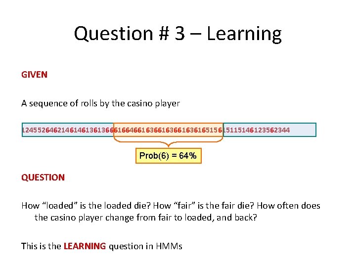
Question # 3 – Learning GIVEN A sequence of rolls by the casino player 12455264621461461361366616646616366163616515615115146123562344 Prob(6) = 64% QUESTION How “loaded” is the loaded die? How “fair” is the fair die? How often does the casino player change from fair to loaded, and back? This is the LEARNING question in HMMs

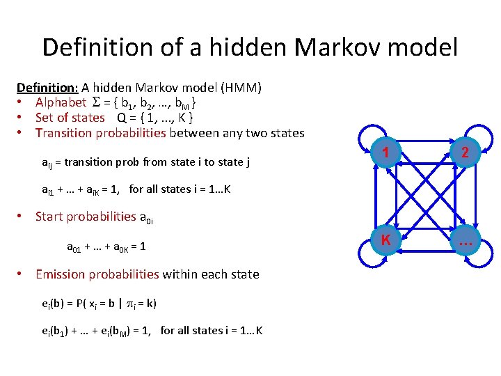
Definition of a hidden Markov model Definition: A hidden Markov model (HMM) • Alphabet = { b 1, b 2, …, b. M } • Set of states Q = { 1, . . . , K } • Transition probabilities between any two states aij = transition prob from state i to state j 1 2 K … ai 1 + … + ai. K = 1, for all states i = 1…K • Start probabilities a 0 i a 01 + … + a 0 K = 1 • Emission probabilities within each state ei(b) = P( xi = b | i = k) ei(b 1) + … + ei(b. M) = 1, for all states i = 1…K

The dishonest casino model 0. 05 0. 95 FAIR P(1|F) = 1/6 P(2|F) = 1/6 P(3|F) = 1/6 P(4|F) = 1/6 P(5|F) = 1/6 P(6|F) = 1/6 0. 95 LOADED 0. 05 P(1|L) = 1/10 P(2|L) = 1/10 P(3|L) = 1/10 P(4|L) = 1/10 P(5|L) = 1/10 P(6|L) = 1/2

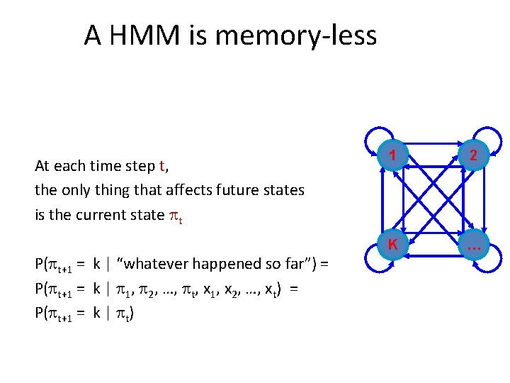
A HMM is memory-less At each time step t, the only thing that affects future states is the current state t P( t+1 = k | “whatever happened so far”) = P( t+1 = k | 1, 2, …, t, x 1, x 2, …, xt) = P( t+1 = k | t) 1 2 K …

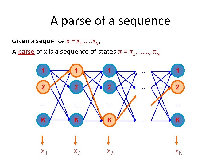
A parse of a sequence Given a sequence x = x 1……x. N, A parse of x is a sequence of states = 1, ……, N 1 1 1 … 1 2 2 2 … … … K K K x 1 x 2 x 3 … … K x. K

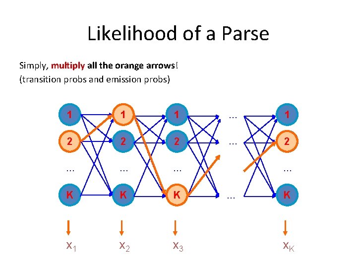
Likelihood of a Parse Simply, multiply all the orange arrows! (transition probs and emission probs) 1 1 1 … 1 2 2 2 … … … K K K x 1 x 2 x 3 … … K x. K

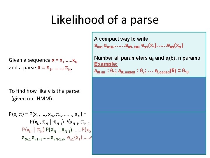
Likelihood of a parse Given a sequence x = x 1……x. N and a parse = 1, ……, N, To find how likely is the parse: (given our HMM) A compact 1 way 1 to write 1 1 … a 0 1 a 1 2……a N-1 N e 1(x 1)……e N(x. N) 2 2 … Number all parameters aij and ei(b); n params … … Example: a 0 Fair : K 1; a 0 Loaded = 18 K : 2; …Ke. Loaded(6)… K Then, count in x and the # of times each parameter j = 1, …, n occurs x 1 x 2 x 3 F(j, x, ) = # parameter j occurs in (x, ) P(x, ) = P(x 1, …, x. N, 1, ……, N) = (call F(. , . ) the feature counts) Then, P(x. N, N | N-1) P(x. N-1, N-1 | N-2)……P(x 2, 2 | 1) P(x 1, 1) = F(j, )x, = ) = P(x. N | N) P( N | N-1) ……P(x 2 |P(x, 2) P( 1 | 1) P( )2 |= 1) P(x j 1 j=1…n a 0 1 a 1 2……a N-1 N e 1(x 1)……e N(x. N) x. K = exp[ j=1…n log( j) F(j, x, )]

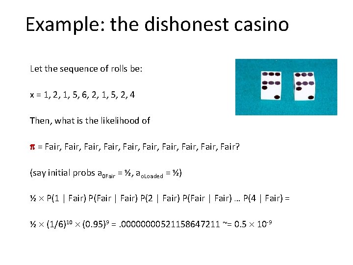
Example: the dishonest casino Let the sequence of rolls be: x = 1, 2, 1, 5, 6, 2, 1, 5, 2, 4 Then, what is the likelihood of = Fair, Fair, Fair, Fair? (say initial probs a 0 Fair = ½, ao. Loaded = ½) ½ P(1 | Fair) P(Fair | Fair) P(2 | Fair) P(Fair | Fair) … P(4 | Fair) = ½ (1/6)10 (0. 95)9 =. 0000521158647211 ~= 0. 5 10 -9

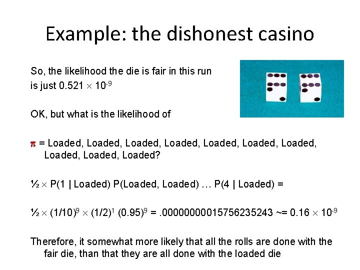
Example: the dishonest casino So, the likelihood the die is fair in this run is just 0. 521 10 -9 OK, but what is the likelihood of = Loaded, Loaded, Loaded, Loaded? ½ P(1 | Loaded) P(Loaded, Loaded) … P(4 | Loaded) = ½ (1/10)9 (1/2)1 (0. 95)9 =. 0000015756235243 ~= 0. 16 10 -9 Therefore, it somewhat more likely that all the rolls are done with the fair die, than that they are all done with the loaded die

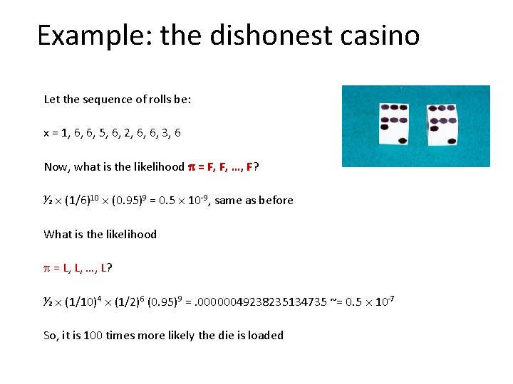
Example: the dishonest casino Let the sequence of rolls be: x = 1, 6, 6, 5, 6, 2, 6, 6, 3, 6 Now, what is the likelihood = F, F, …, F? ½ (1/6)10 (0. 95)9 = 0. 5 10 -9, same as before What is the likelihood = L, L, …, L? ½ (1/10)4 (1/2)6 (0. 95)9 =. 00000049238235134735 ~= 0. 5 10 -7 So, it is 100 times more likely the die is loaded

A+ Model C+ for CGH G+ HMM data Fridlyand et al. (2004) S 1 S 2 S 3 S 4

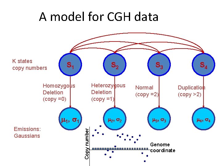
A model for CGH data K states copy numbers S 1 S 2 Heterozygous Deletion (copy =1) Homozygous Deletion (copy =0) 1 , 1 Copy number Emissions: Gaussians 2 , 2 S 3 Normal (copy =2) 3 , 3 Genome coordinate S 4 Duplication (copy >2) 4 , 4

Sources • BJ Raphael, S Volik, C Collins, PA Pevzner - Reconstructing tumor genome architectures. Bioinformatics, 2003 • Raphael and Pevzner. Reconstructing tumor amplisomes. Bioinformatics, 2004 • Olshen et al. Circular binary segmentation for the analysis of array-based DNA copy number data. Biostatistics, 2004. • Lipson, et al. Efficient Calculation of Interval Scores for DNA Copy Number Data Analysis. Journal of Computational Biology, 2006. • Fridyland, et al. Hidden Markov models approach to the analysis of array CGH data. Journal of Multivariate Analysis, 2004 • http: //ai. stanford. edu/~serafim/CS 262_2006/ (HMM slides)