CSCI 200 DATA MINING Introduction to Linear Regression

CSCI 200 DATA MINING Introduction to Linear Regression – Predicting Quality of Wine

Predicting Quality of Wine • Linear Regression is simple and powerful method to analyze data and make predictions • Bordeaux is a region in France popular for producing wine • There are differences in price and quality from year to year that are sometimes very significant • Bordeaux wines are widely believed to taste better when they are older. • There is an incentive to store young wines until they are mature

Predicting Quality of Wine • The main issue: it is hard to determine the quality of the wine when it is so young just by tasting it, since the taste will change significantly by the time it will be consumed • Wine testers and experts taste the wine and then predict which ones will be the best one latest • Question: can we model this process and make stronger predictions •

Predicting Quality of Wine • On March 4, 1990, the New York Times announced that Princeton Professor of Economics Orley Ashenfelter can predict the quality of Bordeaux wine without tasting a single drop. • Ashenfelter's predictions have nothing to do with assessing the aroma of the wine. • They are the results of a mathematical model. • Ashenfelter used a method called linear regression.

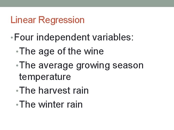
Linear Regression • The methods predicts an outcome variable or dependent variable. • It uses a set independent variables. • Dependent variable: a typical price in 1990 -1991 for Bordeaux wine in an auction. • This approximates quality. • independent variables: age of the wine-- so the older wines are more expensive--and weatherrelated information

Linear Regression • Four independent variables: • The age of the wine • The average growing season temperature • The harvest rain • The winter rain

Quality of Wine – Linear Regression • Professor Ashenfelter believed that his predictions are more accurate than those of the world's most influential wine critic, Robert Parker. • Robert M. Parker Jr. , generally regarded as the most influential wine critic in America, calls Professor Ashenfelter's research ''ludicrous and absurd. ''

Predicting Quality of Wine - Links • http: //www. wine- economics. org/workingpapers/AAWE_WP 0 4. pdf • http: //www. wine-economics. org/ • http: //www. nytimes. com/1990/03/04/us/win e-equation-puts-some-noses-out-ofjoint. html

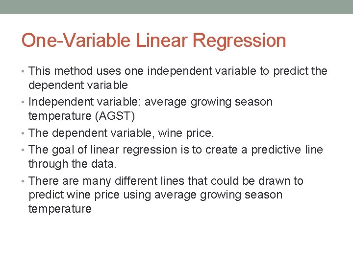
One-Variable Linear Regression • This method uses one independent variable to predict the dependent variable • Independent variable: average growing season temperature (AGST) • The dependent variable, wine price. • The goal of linear regression is to create a predictive line through the data. • There are many different lines that could be drawn to predict wine price using average growing season temperature

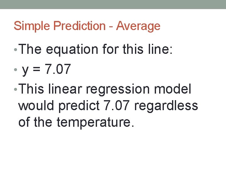
Simple Prediction - Average • The equation for this line: • y = 7. 07 • This linear regression model would predict 7. 07 regardless of the temperature.

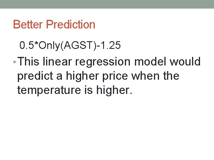
Better Prediction 0. 5*Only(AGST)-1. 25 • This linear regression model would predict a higher price when the temperature is higher.

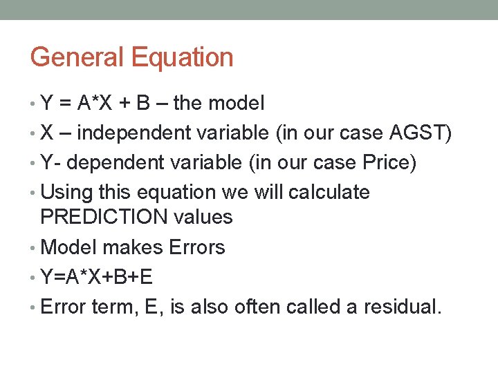
General Equation • Y = A*X + B – the model • X – independent variable (in our case AGST) • Y- dependent variable (in our case Price) • Using this equation we will calculate PREDICTION values • Model makes Errors • Y=A*X+B+E • Error term, E, is also often called a residual.

Y[i]=A*X[i]+B + E[i] • For each observation, i, we have data for the dependent variable Yi and data for the independent variable, Xi. • Using this equation we make a prediction. • This prediction is hopefully close to the true outcome, Yi. • Since the coefficients have to be the same for all data points, i, we often make a small error, E[i] • The best model (choice of A and B) has the smallest error

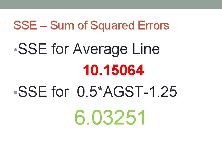
SSE – Sum of Squared Errors • SSE for Average Line 10. 15064 • SSE for 0. 5*AGST-1. 25 6. 03251

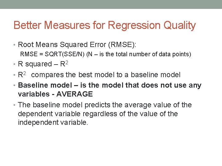
Better Measures for Regression Quality • Root Means Squared Error (RMSE): RMSE = SQRT(SSE/N) (N – is the total number of data points) • R squared – R 2 • R 2 compares the best model to a baseline model • Baseline model – is the model that does not use any variables - AVERAGE • The baseline model predicts the average value of the dependent variable regardless of the value of the independent variable.

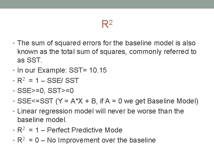
R 2 • The sum of squared errors for the baseline model is also known as the total sum of squares, commonly referred to as SST. • In our Example: SST= 10. 15 • R 2 = 1 – SSE/ SST • SSE>=0, SST>=0 • SSE<=SST (Y = A*X + B, if A = 0 we get Baseline Model) • Linear regression model will never be worse than the baseline model. • R 2 = 1 – Perfect Predictive Mode • R 2 = 0 – No Improvement over the baseline

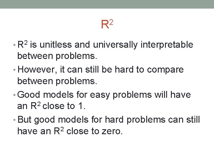
R 2 • R 2 is unitless and universally interpretable between problems. • However, it can still be hard to compare between problems. • Good models for easy problems will have an R 2 close to 1. • But good models for hard problems can still have an R 2 close to zero.

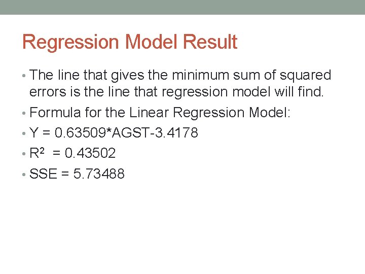
Regression Model Result • The line that gives the minimum sum of squared errors is the line that regression model will find. • Formula for the Linear Regression Model: • Y = 0. 63509*AGST-3. 4178 • R 2 = 0. 43502 • SSE = 5. 73488