CSCE 587 Final Review Rules of Engagement Questions

CSCE 587 Final Review

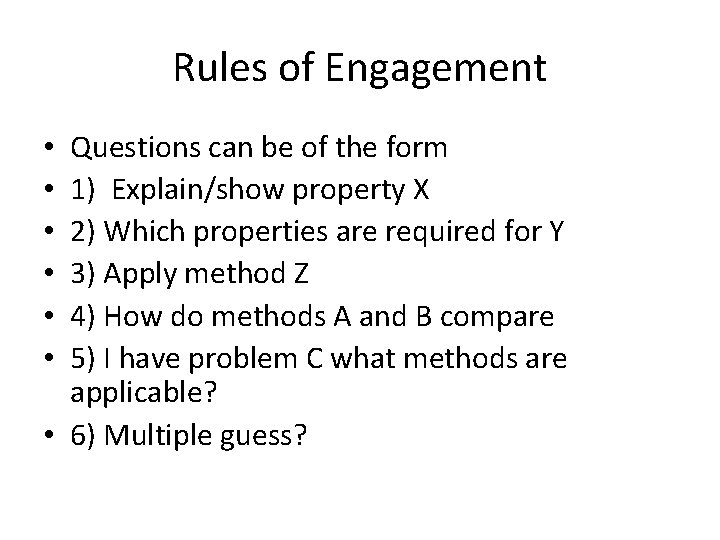
Rules of Engagement Questions can be of the form 1) Explain/show property X 2) Which properties are required for Y 3) Apply method Z 4) How do methods A and B compare 5) I have problem C what methods are applicable? • 6) Multiple guess? • • •

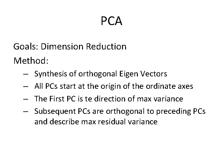
PCA Goals: Dimension Reduction Method: – – Synthesis of orthogonal Eigen Vectors All PCs start at the origin of the ordinate axes The First PC is te direction of max variance Subsequent PCs are orthogonal to preceding PCs and describe max residual variance

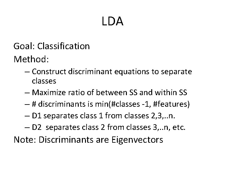
LDA Goal: Classification Method: – Construct discriminant equations to separate classes – Maximize ratio of between SS and within SS – # discriminants is min(#classes -1, #features) – D 1 separates class 1 from classes 2, 3, . . n. – D 2 separates class 2 from classes 3, . . n, etc. Note: Discriminants are Eigenvectors

Time Series Analysis

Modeling a Time Series • Let's model the time series as Yt =Tt +St +Rt, t=1, . . . , n. • Tt: Trend term – Sales of i. Pads steadily increased over the last few years: trending upward. • St: The seasonal term (short term periodicity) – Retail sales fluctuate in a regular pattern over the course of a year. • Typically, sales increase from September through December and decline in January and February. • Rt: Random fluctuation – Noise, or regular high frequency patterns in fluctuation Module 4: Analytics Theory/Methods 6

Stationary Sequences Many time series analyses (Basic Box-Jenkins in particular) assume stationary sequences: – Mean, variance and autocorrelation structure do not change over time – In practice, this often means you must de-trend and seasonally adjust the data – ARIMA in principle can make the data (more) stationary with differencing 7

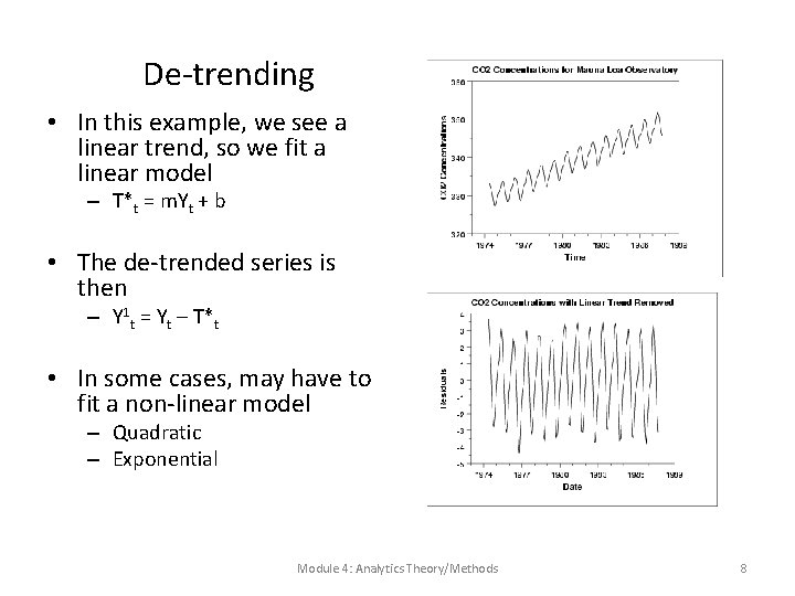
De-trending • In this example, we see a linear trend, so we fit a linear model – T*t = m. Yt + b • The de-trended series is then – Y 1 t = Yt – T*t • In some cases, may have to fit a non-linear model – Quadratic – Exponential Module 4: Analytics Theory/Methods 8

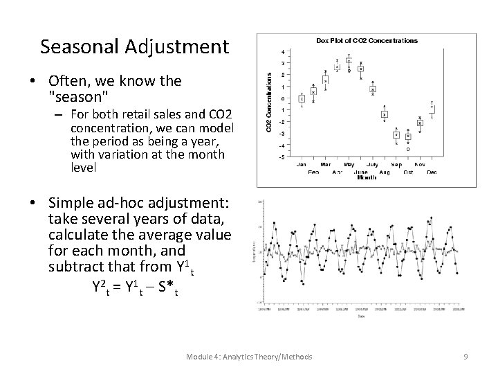
Seasonal Adjustment • Often, we know the "season" – For both retail sales and CO 2 concentration, we can model the period as being a year, with variation at the month level • Simple ad-hoc adjustment: take several years of data, calculate the average value for each month, and subtract that from Y 1 t Y 2 t = Y 1 t – S*t Module 4: Analytics Theory/Methods 9

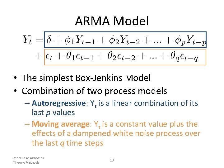
ARMA Model • The simplest Box-Jenkins Model • Combination of two process models – Autoregressive: Yt is a linear combination of its last p values – Moving average: Yt is a constant value plus the effects of a dampened white noise process over the last q time steps Module 4: Analytics Theory/Methods 10

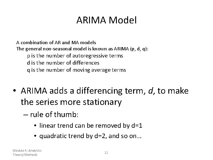
ARIMA Model A combination of AR and MA models The general non-seasonal model is known as ARIMA (p, d, q): p is the number of autoregressive terms d is the number of differences q is the number of moving average terms • ARIMA adds a differencing term, d, to make the series more stationary – rule of thumb: • linear trend can be removed by d=1 • quadratic trend by d=2, and so on… Module 4: Analytics Theory/Methods 11

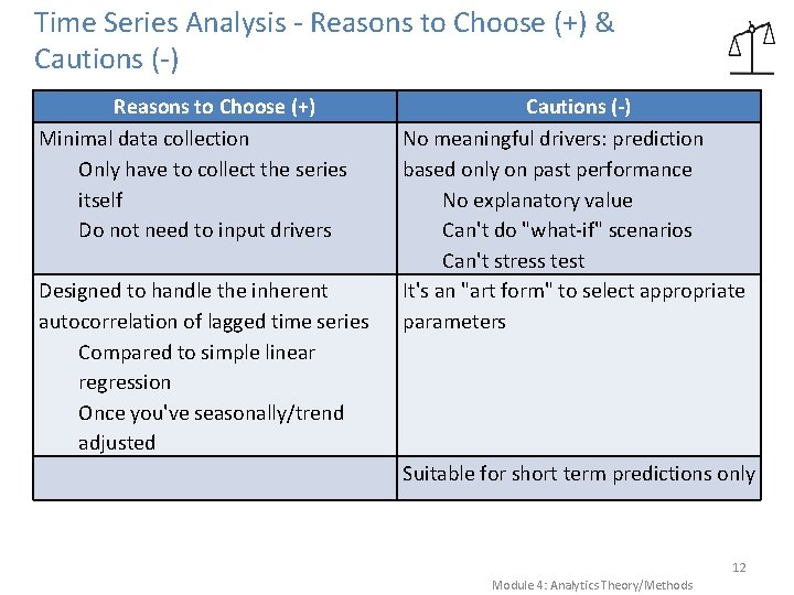
Time Series Analysis - Reasons to Choose (+) & Cautions (-) Reasons to Choose (+) Minimal data collection Only have to collect the series itself Do not need to input drivers Designed to handle the inherent autocorrelation of lagged time series Compared to simple linear regression Once you've seasonally/trend adjusted Cautions (-) No meaningful drivers: prediction based only on past performance No explanatory value Can't do "what-if" scenarios Can't stress test It's an "art form" to select appropriate parameters Suitable for short term predictions only 12 Module 4: Analytics Theory/Methods

Hadoop

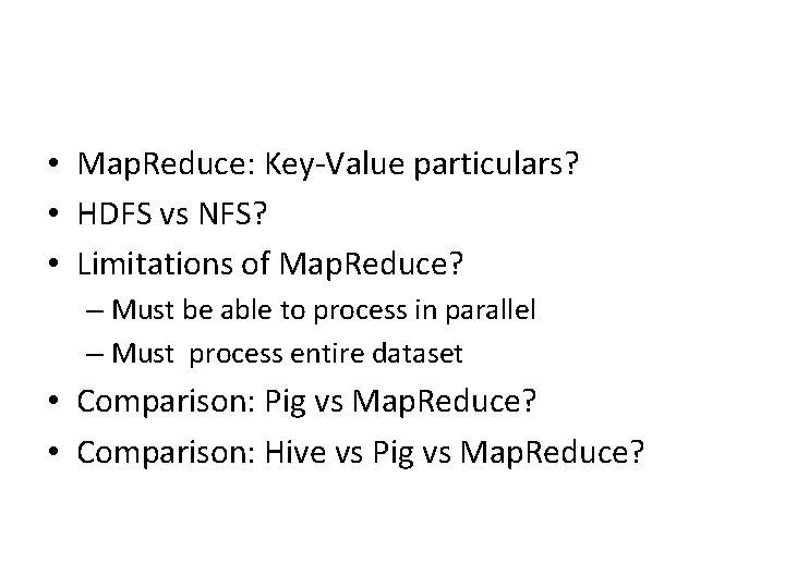
• Map. Reduce: Key-Value particulars? • HDFS vs NFS? • Limitations of Map. Reduce? – Must be able to process in parallel – Must process entire dataset • Comparison: Pig vs Map. Reduce? • Comparison: Hive vs Pig vs Map. Reduce?

Decision Trees CSCE 587

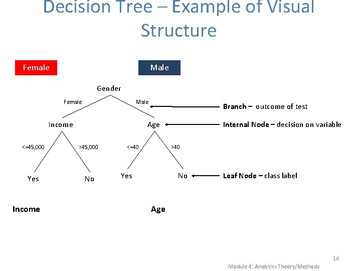
Decision Tree – Example of Visual Structure Female Male Gender Female Male Income Age <=45, 000 >45, 000 Yes No Income Branch – outcome of test <=40 Internal Node – decision on variable >40 Yes No Leaf Node – class label Age 16 Module 4: Analytics Theory/Methods

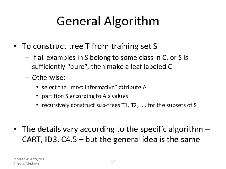
General Algorithm • To construct tree T from training set S – If all examples in S belong to some class in C, or S is sufficiently "pure", then make a leaf labeled C. – Otherwise: • select the “most informative” attribute A • partition S according to A’s values • recursively construct sub-trees T 1, T 2, . . . , for the subsets of S • The details vary according to the specific algorithm – CART, ID 3, C 4. 5 – but the general idea is the same Module 4: Analytics Theory/Methods 17

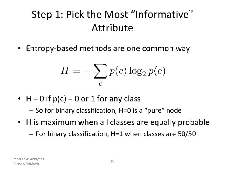
Step 1: Pick the Most “Informative" Attribute • Entropy-based methods are one common way • H = 0 if p(c) = 0 or 1 for any class – So for binary classification, H=0 is a "pure" node • H is maximum when all classes are equally probable – For binary classification, H=1 when classes are 50/50 Module 4: Analytics Theory/Methods 18

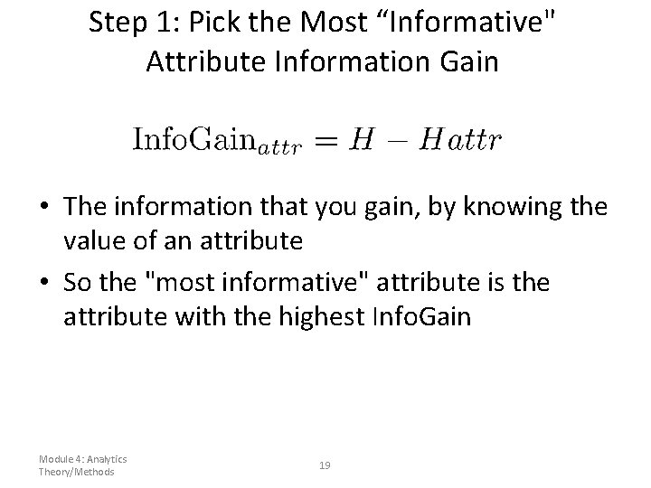
Step 1: Pick the Most “Informative" Attribute Information Gain • The information that you gain, by knowing the value of an attribute • So the "most informative" attribute is the attribute with the highest Info. Gain Module 4: Analytics Theory/Methods 19

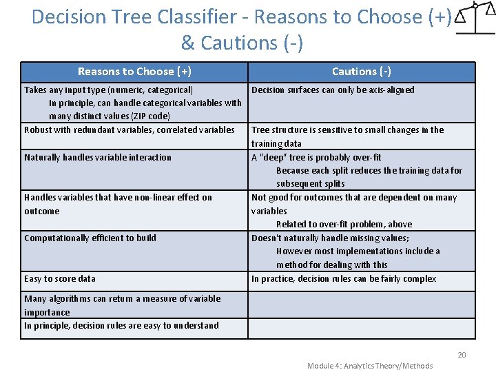
Decision Tree Classifier - Reasons to Choose (+) & Cautions (-) Reasons to Choose (+) Takes any input type (numeric, categorical) In principle, can handle categorical variables with many distinct values (ZIP code) Robust with redundant variables, correlated variables Naturally handles variable interaction Handles variables that have non-linear effect on outcome Computationally efficient to build Easy to score data Cautions (-) Decision surfaces can only be axis-aligned Tree structure is sensitive to small changes in the training data A "deep" tree is probably over-fit Because each split reduces the training data for subsequent splits Not good for outcomes that are dependent on many variables Related to over-fit problem, above Doesn't naturally handle missing values; However most implementations include a method for dealing with this In practice, decision rules can be fairly complex Many algorithms can return a measure of variable importance In principle, decision rules are easy to understand 20 Module 4: Analytics Theory/Methods

K-means Clustering

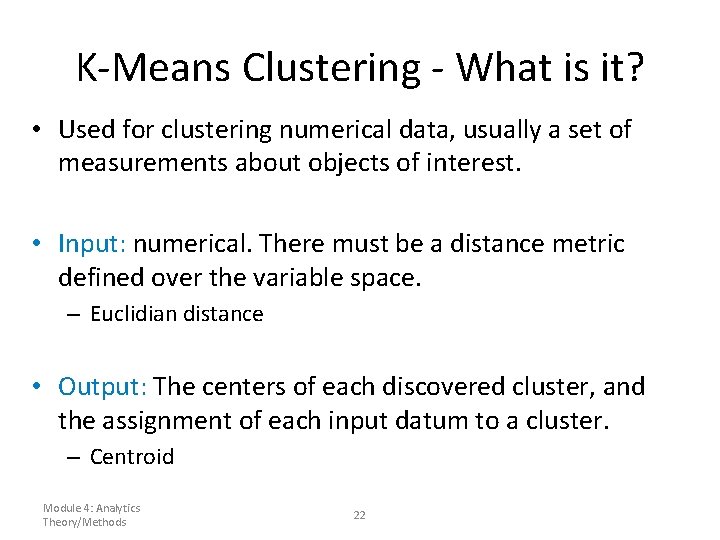
K-Means Clustering - What is it? • Used for clustering numerical data, usually a set of measurements about objects of interest. • Input: numerical. There must be a distance metric defined over the variable space. – Euclidian distance • Output: The centers of each discovered cluster, and the assignment of each input datum to a cluster. – Centroid Module 4: Analytics Theory/Methods 22

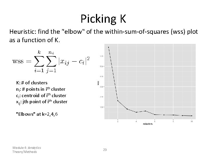
Picking K Heuristic: find the "elbow" of the within-sum-of-squares (wss) plot as a function of K. K: # of clusters ni: # points in ith cluster ci: centroid of ith cluster xij: jth point of ith cluster "Elbows" at k=2, 4, 6 Module 4: Analytics Theory/Methods 23

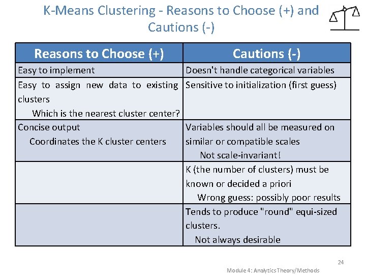
K-Means Clustering - Reasons to Choose (+) and Cautions (-) Reasons to Choose (+) Easy to implement Easy to assign new data to existing clusters Which is the nearest cluster center? Concise output Coordinates the K cluster centers Cautions (-) Doesn't handle categorical variables Sensitive to initialization (first guess) Variables should all be measured on similar or compatible scales Not scale-invariant! K (the number of clusters) must be known or decided a priori Wrong guess: possibly poor results Tends to produce "round" equi-sized clusters. Not always desirable 24 Module 4: Analytics Theory/Methods

Hypothesis Testing CSCE 587

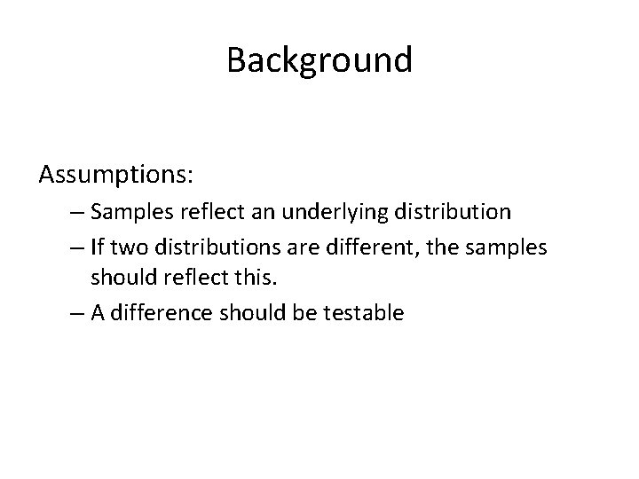
Background Assumptions: – Samples reflect an underlying distribution – If two distributions are different, the samples should reflect this. – A difference should be testable

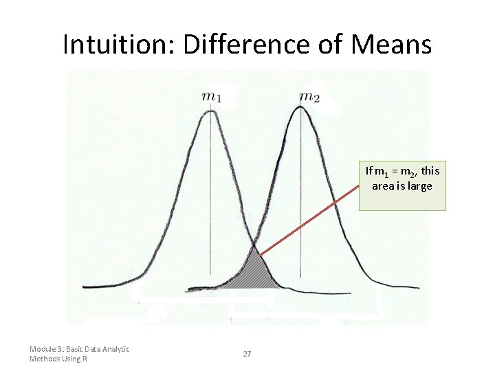
Intuition: Difference of Means If m 1 = m 2, this area is large Module 3: Basic Data Analytic Methods Using R 27

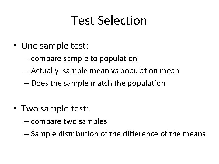
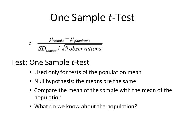
Test Selection • One sample test: – compare sample to population – Actually: sample mean vs population mean – Does the sample match the population • Two sample test: – compare two samples – Sample distribution of the difference of the means

One Sample t-Test: One Sample t-test • Used only for tests of the population mean • Null hypothesis: the means are the same • Compare the mean of the sample with the mean of the population • What do we know about the population?

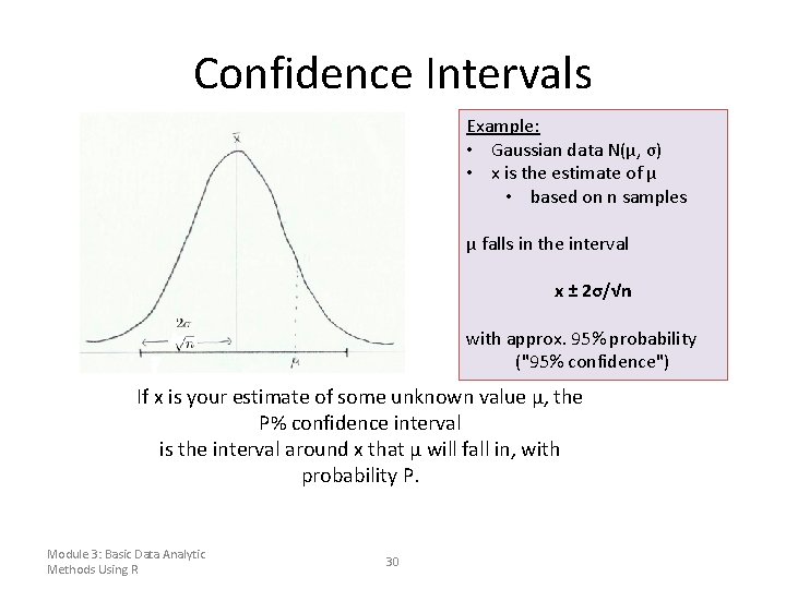
Confidence Intervals Example: • Gaussian data N(μ, σ) • x is the estimate of μ • based on n samples μ falls in the interval x ± 2σ/√n with approx. 95% probability ("95% confidence") If x is your estimate of some unknown value μ, the P% confidence interval is the interval around x that μ will fall in, with probability P. Module 3: Basic Data Analytic Methods Using R 30

Association Rules CSCE 587

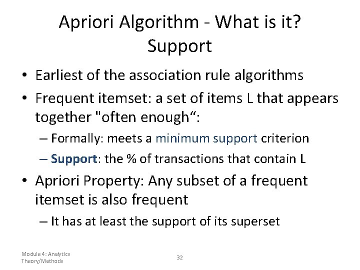
Apriori Algorithm - What is it? Support • Earliest of the association rule algorithms • Frequent itemset: a set of items L that appears together "often enough“: – Formally: meets a minimum support criterion – Support: the % of transactions that contain L • Apriori Property: Any subset of a frequent itemset is also frequent – It has at least the support of its superset Module 4: Analytics Theory/Methods 32

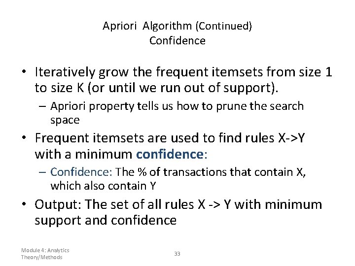
Apriori Algorithm (Continued) Confidence • Iteratively grow the frequent itemsets from size 1 to size K (or until we run out of support). – Apriori property tells us how to prune the search space • Frequent itemsets are used to find rules X->Y with a minimum confidence: – Confidence: The % of transactions that contain X, which also contain Y • Output: The set of all rules X -> Y with minimum support and confidence Module 4: Analytics Theory/Methods 33

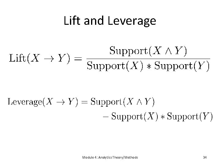
Lift and Leverage Module 4: Analytics Theory/Methods 34

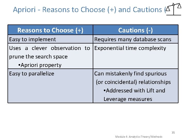
Apriori - Reasons to Choose (+) and Cautions (-) Reasons to Choose (+) Cautions (-) Easy to implement Requires many database scans Uses a clever observation to Exponential time complexity prune the search space • Apriori property Easy to parallelize Can mistakenly find spurious (or coincidental) relationships • Addressed with Lift and Leverage measures 35 Module 4: Analytics Theory/Methods

Linear Regression CSCE 587

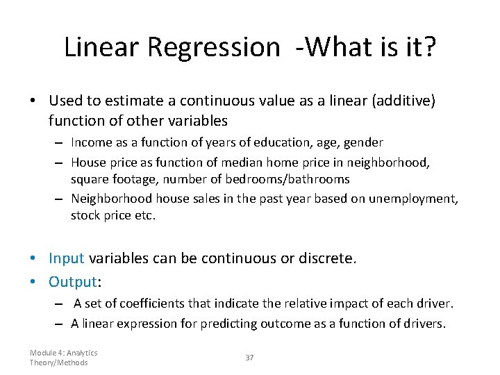
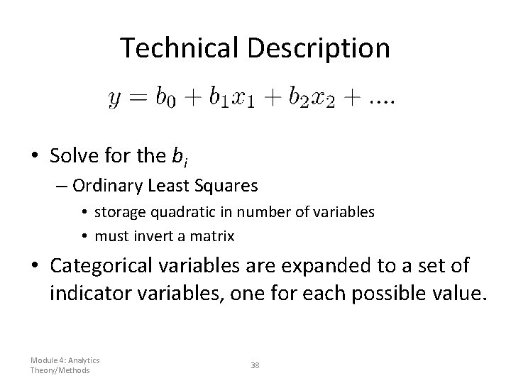
Linear Regression -What is it? • Used to estimate a continuous value as a linear (additive) function of other variables – Income as a function of years of education, age, gender – House price as function of median home price in neighborhood, square footage, number of bedrooms/bathrooms – Neighborhood house sales in the past year based on unemployment, stock price etc. • Input variables can be continuous or discrete. • Output: – A set of coefficients that indicate the relative impact of each driver. – A linear expression for predicting outcome as a function of drivers. Module 4: Analytics Theory/Methods 37

Technical Description • Solve for the bi – Ordinary Least Squares • storage quadratic in number of variables • must invert a matrix • Categorical variables are expanded to a set of indicator variables, one for each possible value. Module 4: Analytics Theory/Methods 38

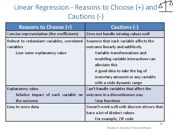
Linear Regression - Reasons to Choose (+) and Cautions (-) Reasons to Choose (+) Concise representation (the coefficients) Cautions (-) Does not handle missing values well Robust to redundant variables, correlated Assumes that each variable affects the variables outcome linearly and additively Lose some explanatory value Variable transformations and modeling variable interactions can alleviate this A good idea to take the log of monetary amounts or any variable with a wide dynamic range Explanatory value Can't handle variables that affect the Relative impact of each variable on outcome in a discontinuous way the outcome Step functions Easy to score data Doesn't work well with discrete drivers that have a lot of distinct values For example, ZIP code 39 Module 4: Analytics Theory/Methods

Logistic Regression CSCE 587

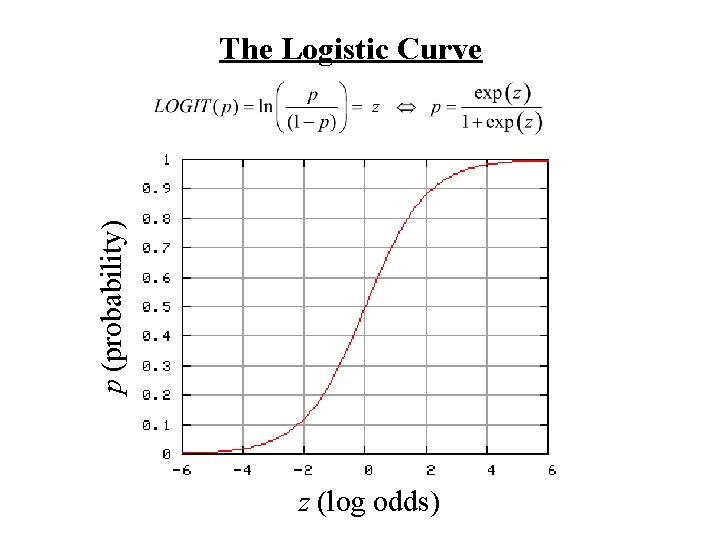
p (probability) The Logistic Curve z (log odds)

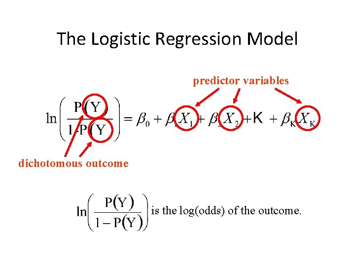
The Logistic Regression Model predictor variables dichotomous outcome is the log(odds) of the outcome.

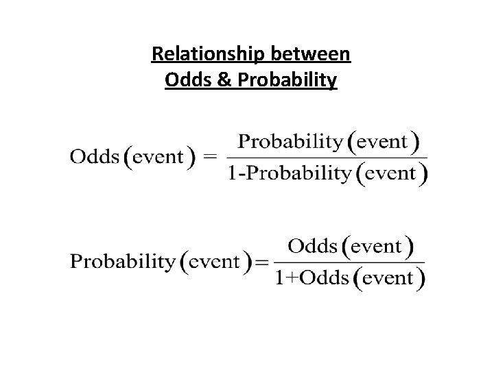
Relationship between Odds & Probability

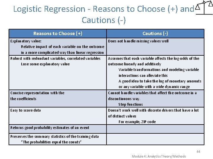
Logistic Regression - Reasons to Choose (+) and Cautions (-) Reasons to Choose (+) Cautions (-) Explanatory value: Does not handle missing values well Relative impact of each variable on the outcome in a more complicated way than linear regression Robust with redundant variables, correlated variables Assumes that each variable affects the log-odds of the Lose some explanatory value outcome linearly and additively Variable transformations and modeling variable interactions can alleviate this A good idea to take the log of monetary amounts or any variable with a wide dynamic range Concise representation with the coefficients Easy to score data Cannot handle variables that affect the outcome in a discontinuous way. Step functions Doesn't work well with discrete drivers that have a lot of distinct values For example, ZIP code Returns good probability estimates of an event Preserves the summary statistics of the training data "The probabilities equal the counts" 44 Module 4: Analytics Theory/Methods

Naïve Bayes CSCE 587

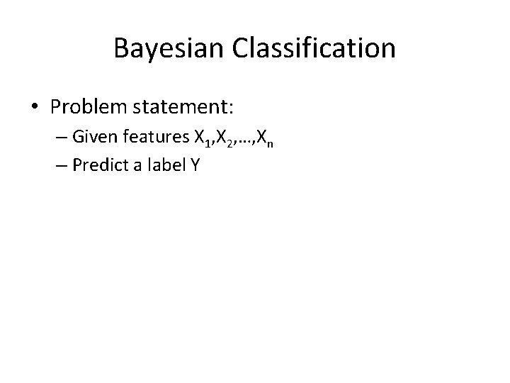
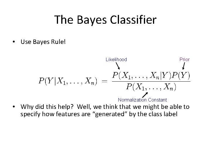
Bayesian Classification • Problem statement: – Given features X 1, X 2, …, Xn – Predict a label Y

The Bayes Classifier • Use Bayes Rule! Likelihood Normalization Constant Prior • Why did this help? Well, we think that we might be able to specify how features are “generated” by the class label

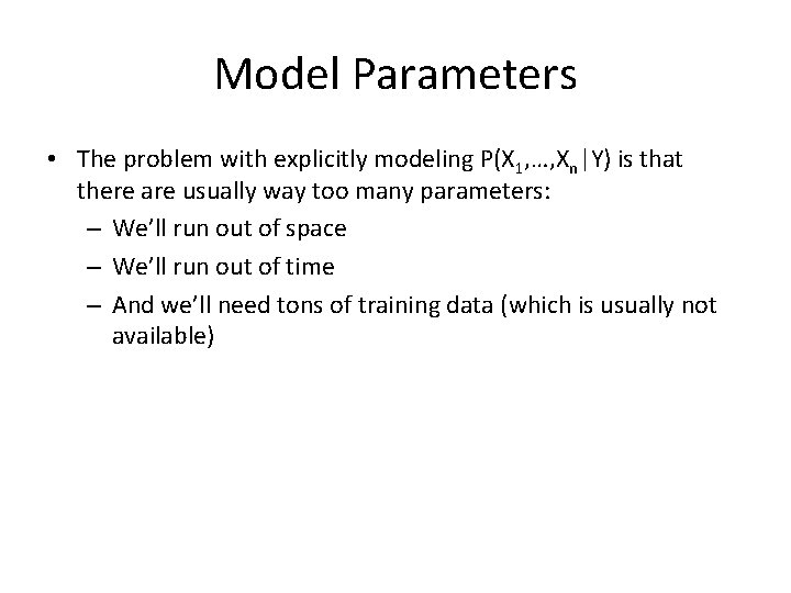
Model Parameters • The problem with explicitly modeling P(X 1, …, Xn|Y) is that there are usually way too many parameters: – We’ll run out of space – We’ll run out of time – And we’ll need tons of training data (which is usually not available)

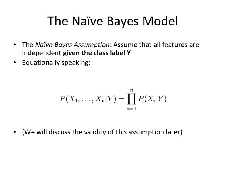
The Naïve Bayes Model • The Naïve Bayes Assumption: Assume that all features are independent given the class label Y • Equationally speaking: • (We will discuss the validity of this assumption later)

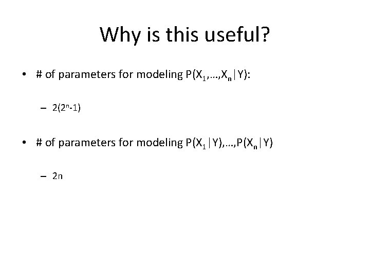
Why is this useful? • # of parameters for modeling P(X 1, …, Xn|Y): – 2(2 n-1) • # of parameters for modeling P(X 1|Y), …, P(Xn|Y) – 2 n

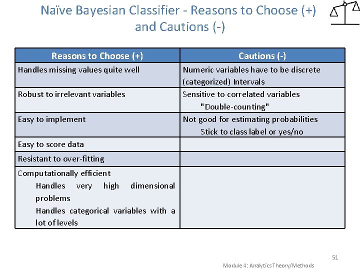
Naïve Bayesian Classifier - Reasons to Choose (+) and Cautions (-) Reasons to Choose (+) Handles missing values quite well Robust to irrelevant variables Easy to implement Cautions (-) Numeric variables have to be discrete (categorized) Intervals Sensitive to correlated variables "Double-counting" Not good for estimating probabilities Stick to class label or yes/no Easy to score data Resistant to over-fitting Computationally efficient Handles very high dimensional problems Handles categorical variables with a lot of levels 51 Module 4: Analytics Theory/Methods

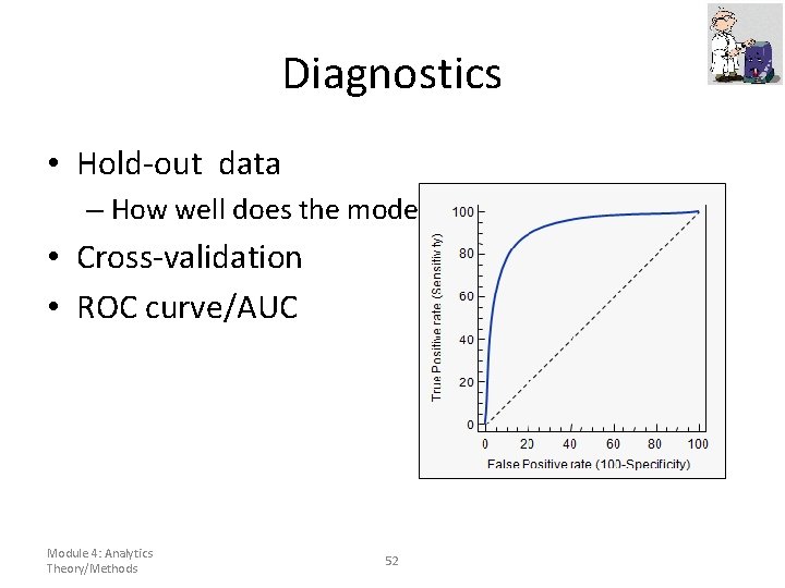
Diagnostics • Hold-out data – How well does the model classify new instances? • Cross-validation • ROC curve/AUC Module 4: Analytics Theory/Methods 52

Conclusion CSCE 587

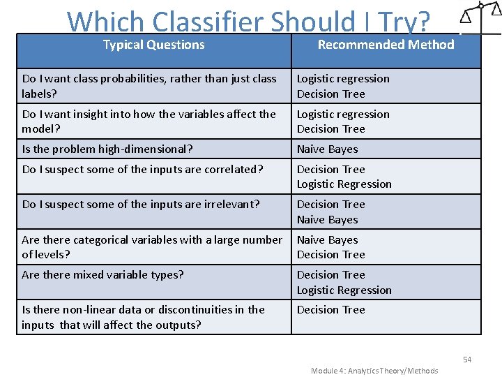
Which Classifier Should I Try? Typical Questions Recommended Method Do I want class probabilities, rather than just class labels? Logistic regression Decision Tree Do I want insight into how the variables affect the model? Logistic regression Decision Tree Is the problem high-dimensional? Naïve Bayes Do I suspect some of the inputs are correlated? Decision Tree Logistic Regression Do I suspect some of the inputs are irrelevant? Decision Tree Naïve Bayes Are there categorical variables with a large number of levels? Naïve Bayes Decision Tree Are there mixed variable types? Decision Tree Logistic Regression Is there non-linear data or discontinuities in the inputs that will affect the outputs? Decision Tree 54 Module 4: Analytics Theory/Methods