CSCE 580 Artificial Intelligence Ch 4 Informed Heuristic
![Acknowledgment • The slides are based on the textbook [AIMA] and other sources, including Acknowledgment • The slides are based on the textbook [AIMA] and other sources, including](https://slidetodoc.com/presentation_image/2823b1377612a641e2f64cb322c2031d/image-2.jpg)
![Review: Tree Search function TREE-SEARCH(problem, fringe) return a solution or failure fringe INSERT(MAKE-NODE(INITIAL-STATE[problem]), fringe) Review: Tree Search function TREE-SEARCH(problem, fringe) return a solution or failure fringe INSERT(MAKE-NODE(INITIAL-STATE[problem]), fringe)](https://slidetodoc.com/presentation_image/2823b1377612a641e2f64cb322c2031d/image-4.jpg)
![Admissibility of A*: A Proof • The following proof is from [P]. Because of Admissibility of A*: A Proof • The following proof is from [P]. Because of](https://slidetodoc.com/presentation_image/2823b1377612a641e2f64cb322c2031d/image-32.jpg)

![Recursive best-first search function RECURSIVE-BEST-FIRST-SEARCH(problem) return a solution or failure return RFBS(problem, MAKE-NODE(INITIAL-STATE[problem]), ∞) Recursive best-first search function RECURSIVE-BEST-FIRST-SEARCH(problem) return a solution or failure return RFBS(problem, MAKE-NODE(INITIAL-STATE[problem]), ∞)](https://slidetodoc.com/presentation_image/2823b1377612a641e2f64cb322c2031d/image-40.jpg)
- Slides: 85

CSCE 580 Artificial Intelligence Ch. 4: Informed (Heuristic) Search and Exploration Fall 2008 Marco Valtorta mgv@cse. sc. edu UNIVERSITY OF SOUTH CAROLINA Department of Computer Science and Engineering
![Acknowledgment The slides are based on the textbook AIMA and other sources including Acknowledgment • The slides are based on the textbook [AIMA] and other sources, including](https://slidetodoc.com/presentation_image/2823b1377612a641e2f64cb322c2031d/image-2.jpg)
Acknowledgment • The slides are based on the textbook [AIMA] and other sources, including other fine textbooks and the accompanying slide sets • The other textbooks I considered are: – David Poole, Alan Mackworth, and Randy Goebel. Computational Intelligence: A Logical Approach. Oxford, 1998 • A second edition (by Poole and Mackworth) is under development. Dr. Poole allowed us to use a draft of it in this course – Ivan Bratko. Prolog Programming for Artificial Intelligence, Third Edition. Addison-Wesley, 2001 • The fourth edition is under development – George F. Luger. Artificial Intelligence: Structures and Strategies for Complex Problem Solving, Sixth Edition. Addison-Welsey, 2009 UNIVERSITY OF SOUTH CAROLINA Department of Computer Science and Engineering

Outline • Informed = use problem-specific knowledge • Which search strategies? – Best-first search and its variants • Heuristic functions? – How to invent them • Local search and optimization – Hill climbing, local beam search, genetic algorithms, … • Local search in continuous spaces • Online search agents UNIVERSITY OF SOUTH CAROLINA Department of Computer Science and Engineering
![Review Tree Search function TREESEARCHproblem fringe return a solution or failure fringe INSERTMAKENODEINITIALSTATEproblem fringe Review: Tree Search function TREE-SEARCH(problem, fringe) return a solution or failure fringe INSERT(MAKE-NODE(INITIAL-STATE[problem]), fringe)](https://slidetodoc.com/presentation_image/2823b1377612a641e2f64cb322c2031d/image-4.jpg)
Review: Tree Search function TREE-SEARCH(problem, fringe) return a solution or failure fringe INSERT(MAKE-NODE(INITIAL-STATE[problem]), fringe) loop do if EMPTY? (fringe) then return failure node REMOVE-FIRST(fringe) if GOAL-TEST[problem] applied to STATE[node] succeeds then return SOLUTION(node) fringe INSERT-ALL(EXPAND(node, problem), fringe) A strategy is defined by picking the order of node expansion UNIVERSITY OF SOUTH CAROLINA Department of Computer Science and Engineering

Best-First Search • General approach of informed search: – Best-first search: node is selected for expansion based on an evaluation function f(n) • Idea: evaluation function measures distance to the goal. – Choose node which appears best • Implementation: – fringe is queue sorted in decreasing order of desirability. – Special cases: greedy search, A* search UNIVERSITY OF SOUTH CAROLINA Department of Computer Science and Engineering

Heuristics and the State-Space Search Heuristic Function • “A rule of thumb, simplification, or educated guess that reduces or limits the search for solutions in domains that are difficult and poorly understood. ” – h(n) = estimated cost of the cheapest path from node n to goal node. – If n is goal then h(n)=0 UNIVERSITY OF SOUTH CAROLINA Department of Computer Science and Engineering

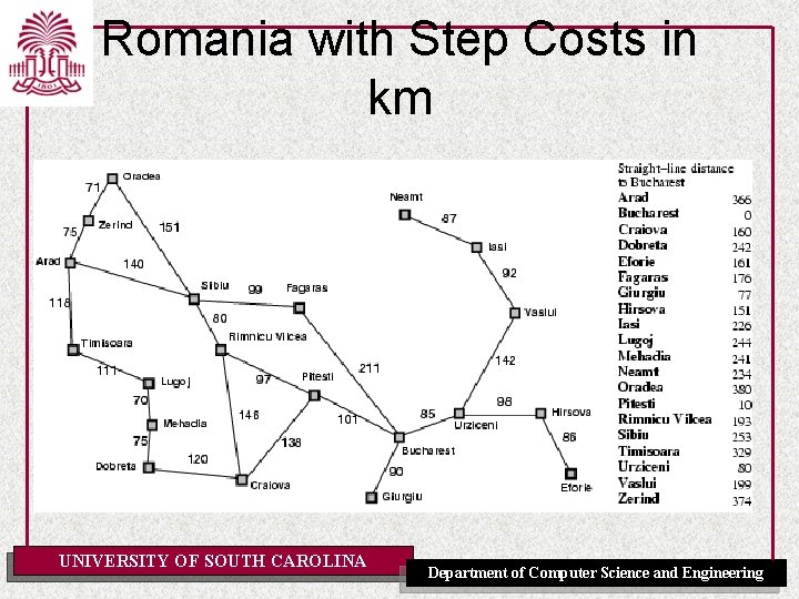
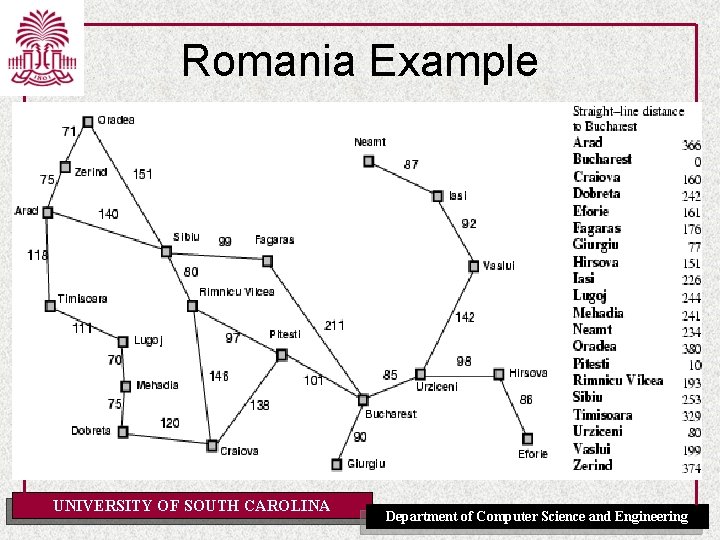
Romania with Step Costs in km UNIVERSITY OF SOUTH CAROLINA Department of Computer Science and Engineering

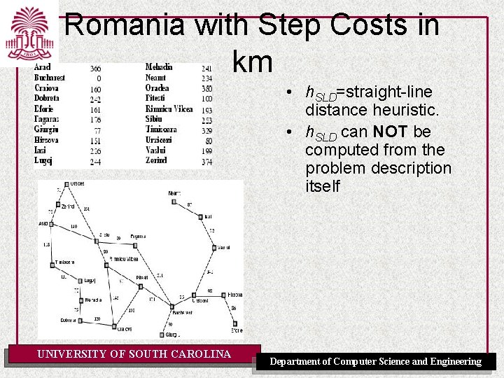
Romania with Step Costs in km • h. SLD=straight-line distance heuristic. • h. SLD can NOT be computed from the problem description itself UNIVERSITY OF SOUTH CAROLINA Department of Computer Science and Engineering

Greedy Best-first Search • Consider f(n)=h(n) – Expand node that is closest to goal = greedy best-first search UNIVERSITY OF SOUTH CAROLINA Department of Computer Science and Engineering

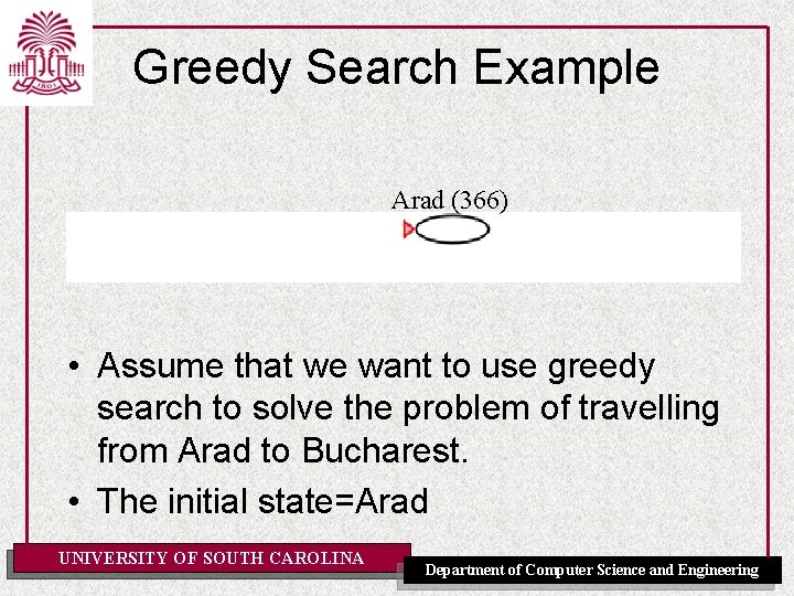
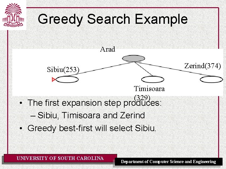
Greedy Search Example Arad (366) • Assume that we want to use greedy search to solve the problem of travelling from Arad to Bucharest. • The initial state=Arad UNIVERSITY OF SOUTH CAROLINA Department of Computer Science and Engineering

Greedy Search Example Arad Zerind(374) Sibiu(253) Timisoara (329) • The first expansion step produces: – Sibiu, Timisoara and Zerind • Greedy best-first will select Sibiu. UNIVERSITY OF SOUTH CAROLINA Department of Computer Science and Engineering

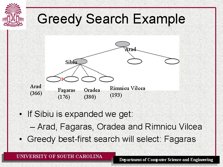
Greedy Search Example Arad Sibiu Arad (366) Fagaras (176) Oradea (380) Rimnicu Vilcea (193) • If Sibiu is expanded we get: – Arad, Fagaras, Oradea and Rimnicu Vilcea • Greedy best-first search will select: Fagaras UNIVERSITY OF SOUTH CAROLINA Department of Computer Science and Engineering

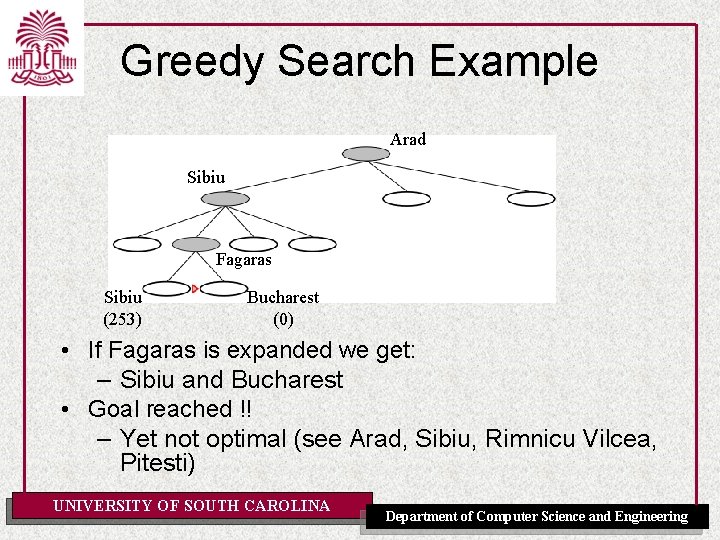
Greedy Search Example Arad Sibiu Fagaras Sibiu (253) Bucharest (0) • If Fagaras is expanded we get: – Sibiu and Bucharest • Goal reached !! – Yet not optimal (see Arad, Sibiu, Rimnicu Vilcea, Pitesti) UNIVERSITY OF SOUTH CAROLINA Department of Computer Science and Engineering

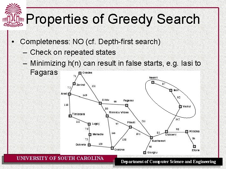
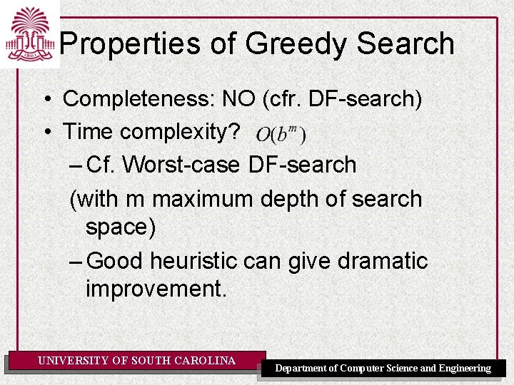
Properties of Greedy Search • Completeness: NO (cf. Depth-first search) – Check on repeated states – Minimizing h(n) can result in false starts, e. g. Iasi to Fagaras UNIVERSITY OF SOUTH CAROLINA Department of Computer Science and Engineering

Properties of Greedy Search • Completeness: NO (cfr. DF-search) • Time complexity? – Cf. Worst-case DF-search (with m maximum depth of search space) – Good heuristic can give dramatic improvement. UNIVERSITY OF SOUTH CAROLINA Department of Computer Science and Engineering

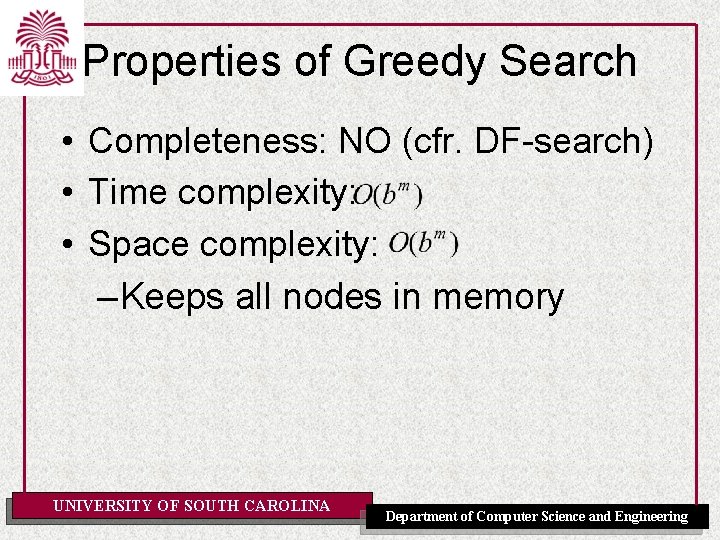
Properties of Greedy Search • Completeness: NO (cfr. DF-search) • Time complexity: • Space complexity: – Keeps all nodes in memory UNIVERSITY OF SOUTH CAROLINA Department of Computer Science and Engineering

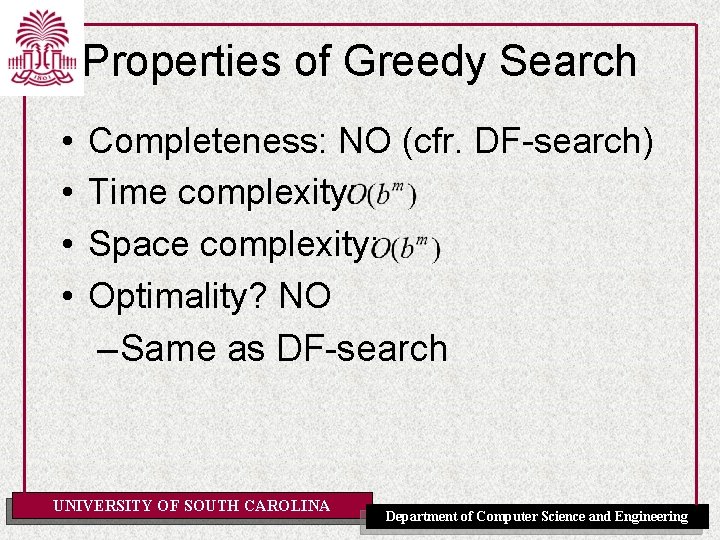
Properties of Greedy Search • • Completeness: NO (cfr. DF-search) Time complexity: Space complexity: Optimality? NO – Same as DF-search UNIVERSITY OF SOUTH CAROLINA Department of Computer Science and Engineering

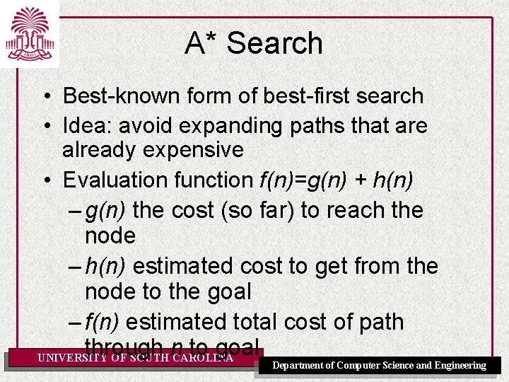
A* Search • Best-known form of best-first search • Idea: avoid expanding paths that are already expensive • Evaluation function f(n)=g(n) + h(n) – g(n) the cost (so far) to reach the node – h(n) estimated cost to get from the node to the goal – f(n) estimated total cost of path through n to goal UNIVERSITY OF SOUTH CAROLINA Department of Computer Science and Engineering

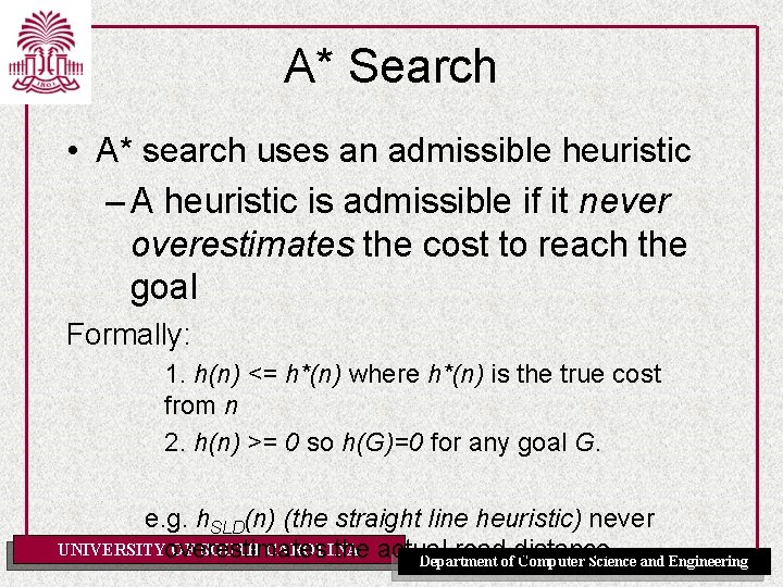
A* Search • A* search uses an admissible heuristic – A heuristic is admissible if it never overestimates the cost to reach the goal Formally: 1. h(n) <= h*(n) where h*(n) is the true cost from n 2. h(n) >= 0 so h(G)=0 for any goal G. e. g. h. SLD(n) (the straight line heuristic) never UNIVERSITYoverestimates OF SOUTH CAROLINA the actual road distance Department of Computer Science and Engineering

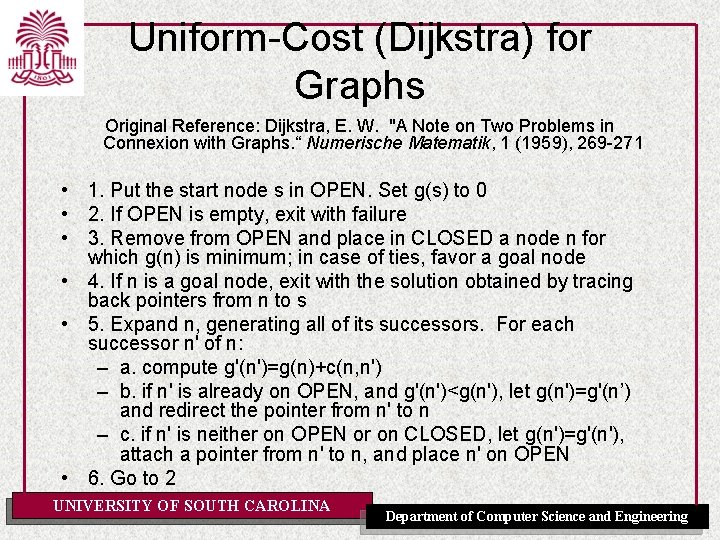
Uniform-Cost (Dijkstra) for Graphs Original Reference: Dijkstra, E. W. "A Note on Two Problems in Connexion with Graphs. “ Numerische Matematik, 1 (1959), 269 -271 • 1. Put the start node s in OPEN. Set g(s) to 0 • 2. If OPEN is empty, exit with failure • 3. Remove from OPEN and place in CLOSED a node n for which g(n) is minimum; in case of ties, favor a goal node • 4. If n is a goal node, exit with the solution obtained by tracing back pointers from n to s • 5. Expand n, generating all of its successors. For each successor n' of n: – a. compute g'(n')=g(n)+c(n, n') – b. if n' is already on OPEN, and g'(n')<g(n'), let g(n')=g'(n’) and redirect the pointer from n' to n – c. if n' is neither on OPEN or on CLOSED, let g(n')=g'(n'), attach a pointer from n' to n, and place n' on OPEN • 6. Go to 2 UNIVERSITY OF SOUTH CAROLINA Department of Computer Science and Engineering

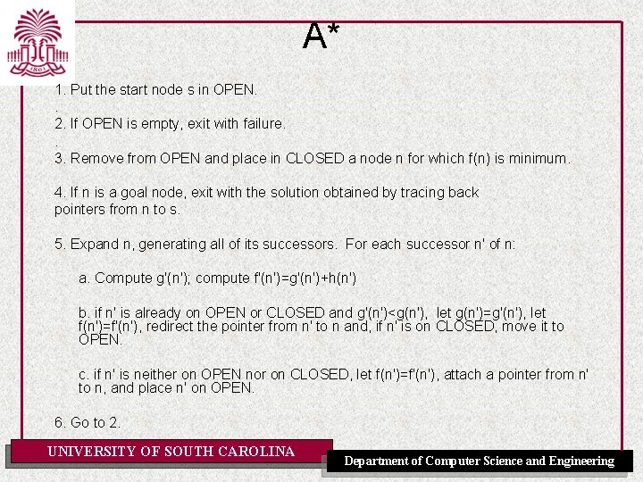
A* 1. Put the start node s in OPEN. . 2. If OPEN is empty, exit with failure. . 3. Remove from OPEN and place in CLOSED a node n for which f(n) is minimum. 4. If n is a goal node, exit with the solution obtained by tracing back pointers from n to s. 5. Expand n, generating all of its successors. For each successor n' of n: a. Compute g'(n'); compute f'(n')=g'(n')+h(n') b. if n' is already on OPEN or CLOSED and g'(n')<g(n'), let g(n')=g'(n'), let f(n')=f'(n'), redirect the pointer from n' to n and, if n' is on CLOSED, move it to OPEN. c. if n' is neither on OPEN nor on CLOSED, let f(n')=f'(n'), attach a pointer from n' to n, and place n' on OPEN. 6. Go to 2. UNIVERSITY OF SOUTH CAROLINA Department of Computer Science and Engineering

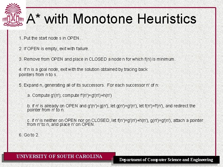
A* with Monotone Heuristics 1. Put the start node s in OPEN. 2. If OPEN is empty, exit with failure. 3. Remove from OPEN and place in CLOSED a node n for which f(n) is minimum. 4. If n is a goal node, exit with the solution obtained by tracing back pointers from n to s. 5. Expand n, generating all of its successors. For each successor n' of n: a. Compute g'(n'); compute f'(n')=g'(n')+h(n') b. if n' is already on OPEN and g'(n')<g(n'), let g(n')=g'(n'), let f(n')=f'(n'), and redirect the pointer from n' to n. c. if n' is neither on OPEN nor on CLOSED, let f(n')=g'(n')+h(n'), g(n')=g'(n'), attach a pointer from n' to n, and place n' on OPEN. 6. Go to 2. UNIVERSITY OF SOUTH CAROLINA Department of Computer Science and Engineering

Romania Example UNIVERSITY OF SOUTH CAROLINA Department of Computer Science and Engineering

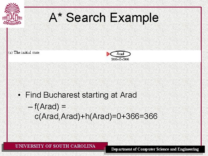
A* Search Example • Find Bucharest starting at Arad – f(Arad) = c(Arad, Arad)+h(Arad)=0+366=366 UNIVERSITY OF SOUTH CAROLINA Department of Computer Science and Engineering

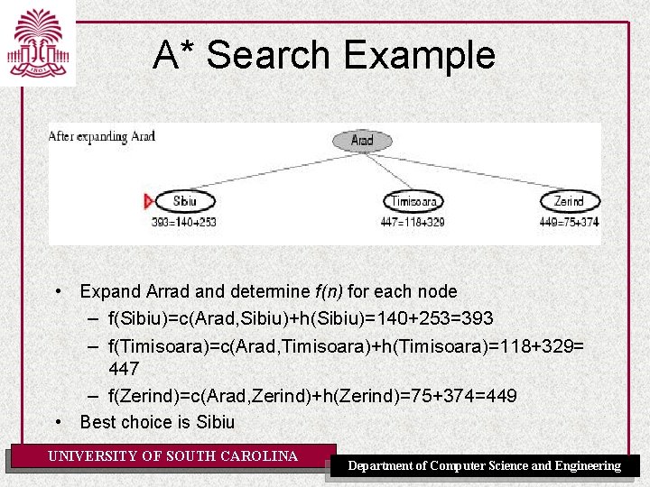
A* Search Example • Expand Arrad and determine f(n) for each node – f(Sibiu)=c(Arad, Sibiu)+h(Sibiu)=140+253=393 – f(Timisoara)=c(Arad, Timisoara)+h(Timisoara)=118+329= 447 – f(Zerind)=c(Arad, Zerind)+h(Zerind)=75+374=449 • Best choice is Sibiu UNIVERSITY OF SOUTH CAROLINA Department of Computer Science and Engineering

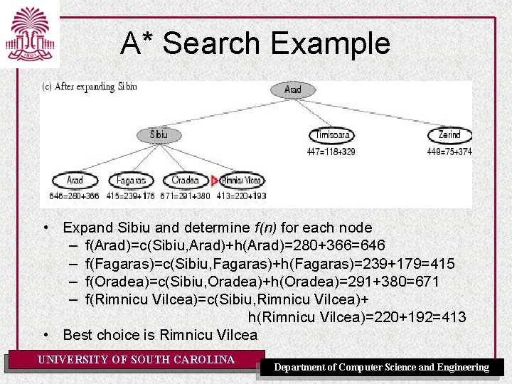
A* Search Example • Expand Sibiu and determine f(n) for each node – f(Arad)=c(Sibiu, Arad)+h(Arad)=280+366=646 – f(Fagaras)=c(Sibiu, Fagaras)+h(Fagaras)=239+179=415 – f(Oradea)=c(Sibiu, Oradea)+h(Oradea)=291+380=671 – f(Rimnicu Vilcea)=c(Sibiu, Rimnicu Vilcea)+ h(Rimnicu Vilcea)=220+192=413 • Best choice is Rimnicu Vilcea UNIVERSITY OF SOUTH CAROLINA Department of Computer Science and Engineering

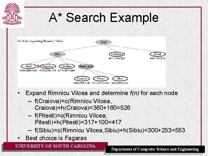
A* Search Example • Expand Rimnicu Vilcea and determine f(n) for each node – f(Craiova)=c(Rimnicu Vilcea, Craiova)+h(Craiova)=360+160=526 – f(Pitesti)=c(Rimnicu Vilcea, Pitesti)+h(Pitesti)=317+100=417 – f(Sibiu)=c(Rimnicu Vilcea, Sibiu)+h(Sibiu)=300+253=553 • Best choice is Fagaras UNIVERSITY OF SOUTH CAROLINA Department of Computer Science and Engineering

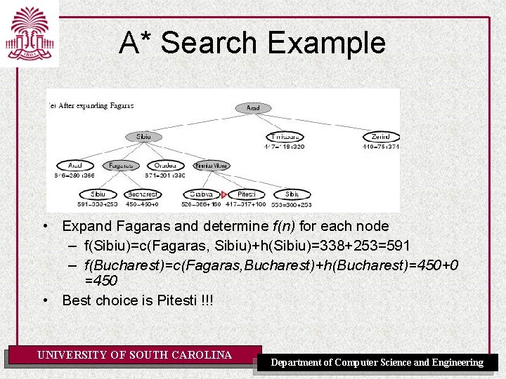
A* Search Example • Expand Fagaras and determine f(n) for each node – f(Sibiu)=c(Fagaras, Sibiu)+h(Sibiu)=338+253=591 – f(Bucharest)=c(Fagaras, Bucharest)+h(Bucharest)=450+0 =450 • Best choice is Pitesti !!! UNIVERSITY OF SOUTH CAROLINA Department of Computer Science and Engineering

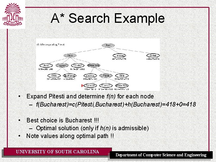
A* Search Example • Expand Pitesti and determine f(n) for each node – f(Bucharest)=c(Pitesti, Bucharest)+h(Bucharest)=418+0=418 • Best choice is Bucharest !!! – Optimal solution (only if h(n) is admissible) • Note values along optimal path !! UNIVERSITY OF SOUTH CAROLINA Department of Computer Science and Engineering

Admissible Heuristics and Search Algorithms • A heuristic h(n) is admissible if for every node n, h(n) ≤ h*(n), where h*(n) is the true cost to reach the goal state from n • An admissible heuristic never overestimates the cost to reach the goal, i. e. , it is optimistic • Example: h. SLD(n) (never overestimates the actual road distance) • A search algorithm is admissible if it returns an optimal solution path – [AIMA] calls such an algorithm optimal, instead of admissible • Theorem: If h(n) is admissible, A* (as presented in this set of slides) is admissible on graphs UNIVERSITY OF SOUTH CAROLINA Department of Computer Science and Engineering

Admissibility of A* • See Section 3. 1. 3 of: Judea Pearl. Heuristics: Intelligent Search Strategies for Computer Problem Solving. Addison-Wesley, 1984. – Especially Lemma 1 and Theorem 2 (pp. 77 -78) • Note that admissibility of A* does not require monotonicity of the heuristics. [AIMA] claims otherwise on p. 99. The confusion is probably due to the fact that admissibility only requires an optimal solution to be returned for a goal node (for which h=0), rather than for every node that is CLOSED • A* finds shortest paths to every node it closes with monotone (consistent) heuristics UNIVERSITY OF SOUTH CAROLINA Department of Computer Science and Engineering
![Admissibility of A A Proof The following proof is from P Because of Admissibility of A*: A Proof • The following proof is from [P]. Because of](https://slidetodoc.com/presentation_image/2823b1377612a641e2f64cb322c2031d/image-32.jpg)
Admissibility of A*: A Proof • The following proof is from [P]. Because of all the undefined terms, we should consider it a proof sketch. • The first path to a goal selected is an optimal path. The f-value for any node on an optimal solution path is less than or equal to the f-value of an optimal solution. This is because h is an underestimate of the actual cost from a node to a goal. Thus the f-value of a node on an optimal solution path is less than the fvalue for any non-optimal solution. Thus a nonoptimal solution can never be chosen while there is a node on the frontier that leads to an optimal solution (as an element with minimum f-value is chosen at each step). So before we can select a non-optimal solution, you will have to pick all of the nodes on an optimal path, including each of the optimal solutions. UNIVERSITY OF SOUTH CAROLINA Department of Computer Science and Engineering

Admissibility of A* • See Section 3. 1. 3 of: Judea Pearl. Heuristics: Intelligent Search Strategies for Computer Problem Solving. Addison-Wesley, 1984. – Especially Lemma 1 and Theorem 2 (pp. 77 -78) • Note that admissibility of A* does not require monotonicity of the heuristics. [AIMA] claims otherwise on p. 99. The confusion is probably due to the fact that admissibility only requires an optimal solution to be returned for a goal node (for which h=0), rather than for every node that is CLOSED • A* finds shortest paths to every node it closes with monotone (consistent) heuristics UNIVERSITY OF SOUTH CAROLINA Department of Computer Science and Engineering

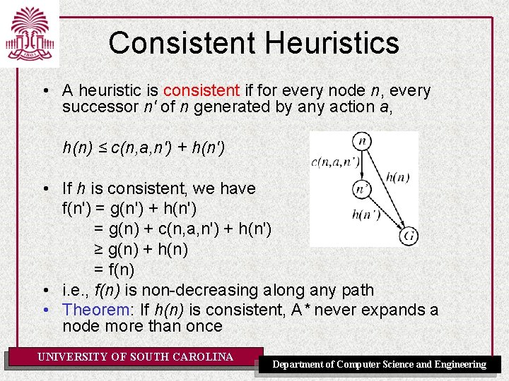
Consistent Heuristics • A heuristic is consistent if for every node n, every successor n' of n generated by any action a, h(n) ≤ c(n, a, n') + h(n') • If h is consistent, we have f(n') = g(n') + h(n') = g(n) + c(n, a, n') + h(n') ≥ g(n) + h(n) = f(n) • i. e. , f(n) is non-decreasing along any path • Theorem: If h(n) is consistent, A* never expands a node more than once UNIVERSITY OF SOUTH CAROLINA Department of Computer Science and Engineering

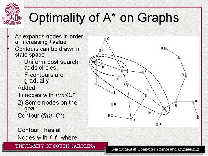
Optimality of A* on Graphs • A* expands nodes in order of increasing f value • Contours can be drawn in state space – Uniform-cost search adds circles. – F-contours are gradually Added: 1) nodes with f(n)<C* 2) Some nodes on the goal Contour (f(n)=C*) Contour I has all Nodes with f=fi, where fi < fi+1 OF SOUTH CAROLINA UNIVERSITY Department of Computer Science and Engineering

A* search, evaluation • Completeness: YES • Time complexity: – Number of nodes expanded is still exponential in the length of the solution. UNIVERSITY OF SOUTH CAROLINA Department of Computer Science and Engineering

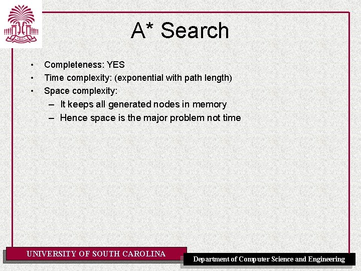
A* Search • • • Completeness: YES Time complexity: (exponential with path length) Space complexity: – It keeps all generated nodes in memory – Hence space is the major problem not time UNIVERSITY OF SOUTH CAROLINA Department of Computer Science and Engineering

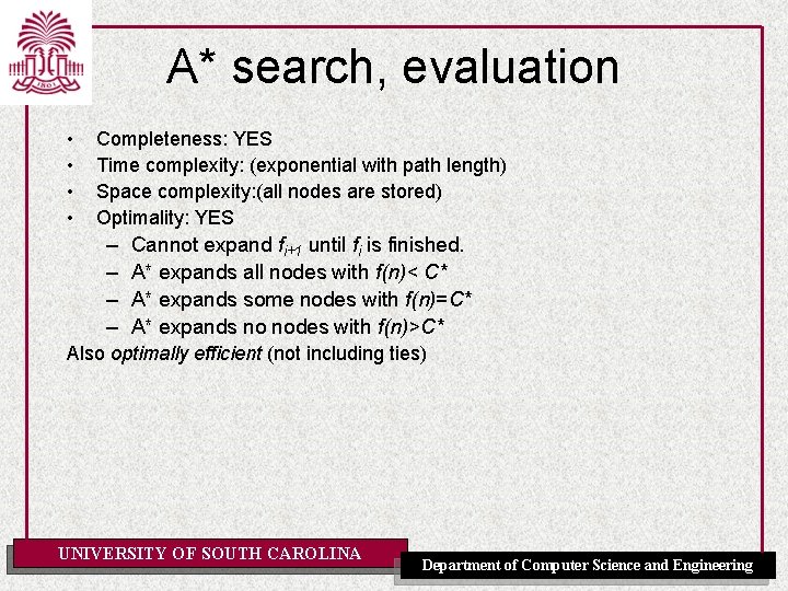
A* search, evaluation • • Completeness: YES Time complexity: (exponential with path length) Space complexity: (all nodes are stored) Optimality: YES – – Cannot expand fi+1 until fi is finished. A* expands all nodes with f(n)< C* A* expands some nodes with f(n)=C* A* expands no nodes with f(n)>C* Also optimally efficient (not including ties) UNIVERSITY OF SOUTH CAROLINA Department of Computer Science and Engineering

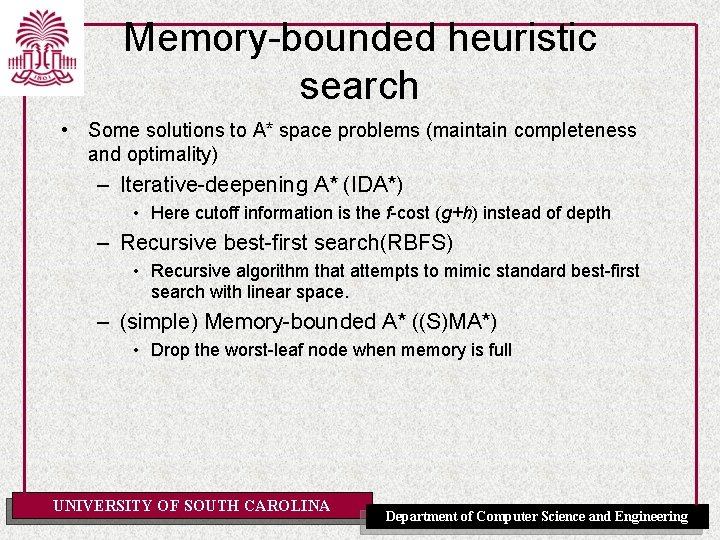
Memory-bounded heuristic search • Some solutions to A* space problems (maintain completeness and optimality) – Iterative-deepening A* (IDA*) • Here cutoff information is the f-cost (g+h) instead of depth – Recursive best-first search(RBFS) • Recursive algorithm that attempts to mimic standard best-first search with linear space. – (simple) Memory-bounded A* ((S)MA*) • Drop the worst-leaf node when memory is full UNIVERSITY OF SOUTH CAROLINA Department of Computer Science and Engineering
![Recursive bestfirst search function RECURSIVEBESTFIRSTSEARCHproblem return a solution or failure return RFBSproblem MAKENODEINITIALSTATEproblem Recursive best-first search function RECURSIVE-BEST-FIRST-SEARCH(problem) return a solution or failure return RFBS(problem, MAKE-NODE(INITIAL-STATE[problem]), ∞)](https://slidetodoc.com/presentation_image/2823b1377612a641e2f64cb322c2031d/image-40.jpg)
Recursive best-first search function RECURSIVE-BEST-FIRST-SEARCH(problem) return a solution or failure return RFBS(problem, MAKE-NODE(INITIAL-STATE[problem]), ∞) function RFBS( problem, node, f_limit) return a solution or failure and a new f-cost limit if GOAL-TEST[problem](STATE[node]) then return node successors EXPAND(node, problem) if successors is empty then return failure, ∞ for each s in successors do f [s] max(g(s) + h(s), f [node]) repeat best the lowest f-value node in successors if f [best] > f_limit then return failure, f [best] alternative the second lowest f-value among successors result, f [best] RBFS(problem, best, min(f_limit, alternative)) if result failure then return result UNIVERSITY OF SOUTH CAROLINA Department of Computer Science and Engineering

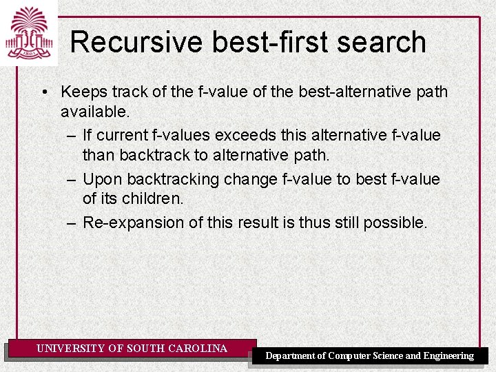
Recursive best-first search • Keeps track of the f-value of the best-alternative path available. – If current f-values exceeds this alternative f-value than backtrack to alternative path. – Upon backtracking change f-value to best f-value of its children. – Re-expansion of this result is thus still possible. UNIVERSITY OF SOUTH CAROLINA Department of Computer Science and Engineering

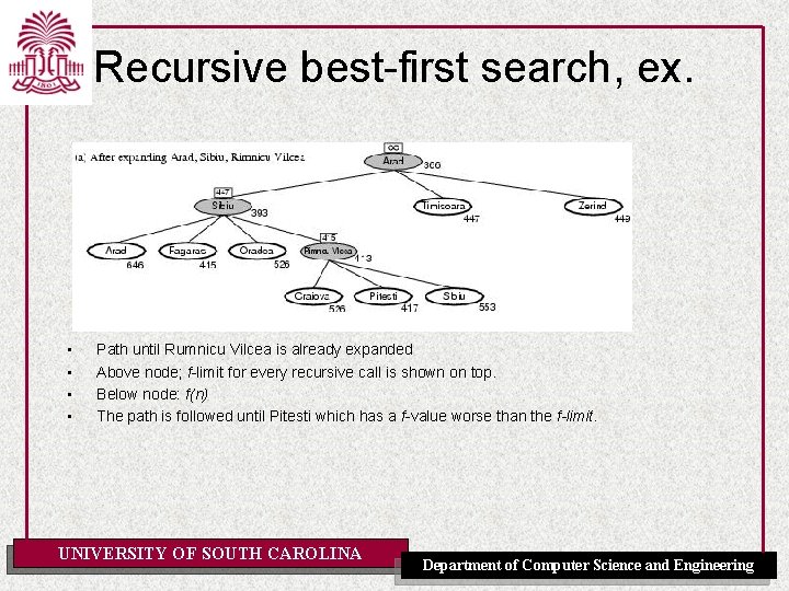
Recursive best-first search, ex. • • Path until Rumnicu Vilcea is already expanded Above node; f-limit for every recursive call is shown on top. Below node: f(n) The path is followed until Pitesti which has a f-value worse than the f-limit. UNIVERSITY OF SOUTH CAROLINA Department of Computer Science and Engineering

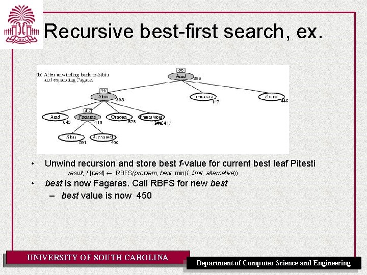
Recursive best-first search, ex. • Unwind recursion and store best f-value for current best leaf Pitesti result, f [best] RBFS(problem, best, min(f_limit, alternative)) • best is now Fagaras. Call RBFS for new best – best value is now 450 UNIVERSITY OF SOUTH CAROLINA Department of Computer Science and Engineering

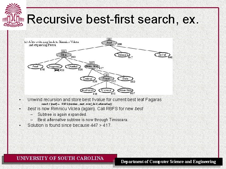
Recursive best-first search, ex. • Unwind recursion and store best f-value for current best leaf Fagaras result, f [best] RBFS(problem, best, min(f_limit, alternative)) • • best is now Rimnicu Viclea (again). Call RBFS for new best – Subtree is again expanded. – Best alternative subtree is now through Timisoara. Solution is found since because 447 > 417. UNIVERSITY OF SOUTH CAROLINA Department of Computer Science and Engineering

RBFS evaluation • RBFS is a bit more efficient than IDA* – Still excessive node generation (mind changes) • • Like A*, optimal if h(n) is admissible Space complexity is O(bd). – IDA* retains only one single number (the current f-cost limit) • Time complexity difficult to characterize – Depends on accuracy if h(n) and how often best path changes. • IDA* en RBFS suffer from too little memory. UNIVERSITY OF SOUTH CAROLINA Department of Computer Science and Engineering

(Simplified) Memory-bounded A* • Use all available memory. – I. e. expand best leafs until available memory is full – When full, SMA* drops worst leaf node (highest f-value) – Like RFBS backup forgotten node to its parent • What if all leaves have the same f-value? – Same node could be selected for expansion and deletion. – SMA* solves this by expanding newest best leaf and deleting oldest worst leaf. • SMA* is complete if solution is reachable, optimal if optimal solution is reachable. UNIVERSITY OF SOUTH CAROLINA Department of Computer Science and Engineering

Learning to search better • • All previous algorithms use fixed strategies. Agents can learn to improve their search by exploiting the meta-level state space. – Each meta-level state is a internal (computational) state of a program that is searching in the object-level state space. – In A* such a state consists of the current search tree • A meta-level learning algorithm from experiences at the meta-level. UNIVERSITY OF SOUTH CAROLINA Department of Computer Science and Engineering

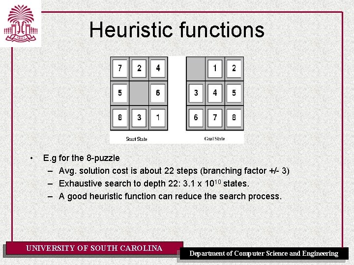
Heuristic functions • E. g for the 8 -puzzle – Avg. solution cost is about 22 steps (branching factor +/- 3) – Exhaustive search to depth 22: 3. 1 x 10¹⁰ states. – A good heuristic function can reduce the search process. UNIVERSITY OF SOUTH CAROLINA Department of Computer Science and Engineering

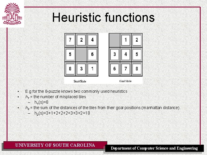
Heuristic functions • • • E. g for the 8 -puzzle knows two commonly used heuristics h 1 = the number of misplaced tiles – h 1(s)=8 h 2 = the sum of the distances of the tiles from their goal positions (manhattan distance). – h 2(s)=3+1+2+2+2+3+3+2=18 UNIVERSITY OF SOUTH CAROLINA Department of Computer Science and Engineering

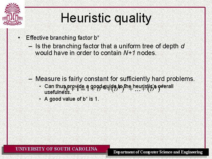
Heuristic quality • Effective branching factor b* – Is the branching factor that a uniform tree of depth d would have in order to contain N+1 nodes. – Measure is fairly constant for sufficiently hard problems. • Can thus provide a good guide to the heuristic’s overall usefulness. • A good value of b* is 1. UNIVERSITY OF SOUTH CAROLINA Department of Computer Science and Engineering

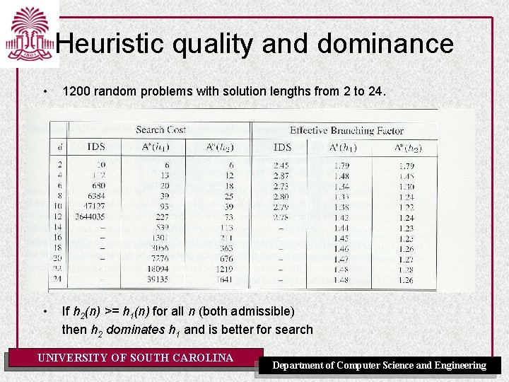
Heuristic quality and dominance • 1200 random problems with solution lengths from 2 to 24. • If h 2(n) >= h 1(n) for all n (both admissible) then h 2 dominates h 1 and is better for search UNIVERSITY OF SOUTH CAROLINA Department of Computer Science and Engineering

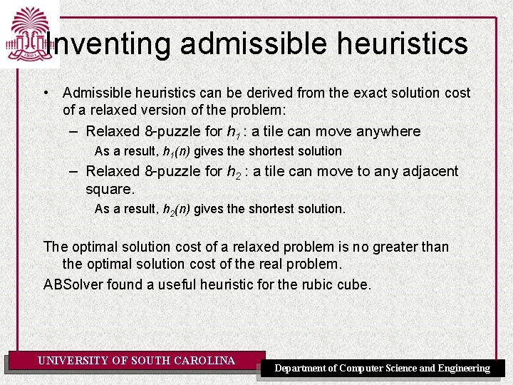
Inventing admissible heuristics • Admissible heuristics can be derived from the exact solution cost of a relaxed version of the problem: – Relaxed 8 -puzzle for h 1 : a tile can move anywhere As a result, h 1(n) gives the shortest solution – Relaxed 8 -puzzle for h 2 : a tile can move to any adjacent square. As a result, h 2(n) gives the shortest solution. The optimal solution cost of a relaxed problem is no greater than the optimal solution cost of the real problem. ABSolver found a useful heuristic for the rubic cube. UNIVERSITY OF SOUTH CAROLINA Department of Computer Science and Engineering

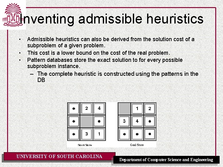
Inventing admissible heuristics • • • Admissible heuristics can also be derived from the solution cost of a subproblem of a given problem. This cost is a lower bound on the cost of the real problem. Pattern databases store the exact solution to for every possible subproblem instance. – The complete heuristic is constructed using the patterns in the DB UNIVERSITY OF SOUTH CAROLINA Department of Computer Science and Engineering

Inventing admissible heuristics • Another way to find an admissible heuristic is through learning from experience: – Experience = solving lots of 8 -puzzles – An inductive learning algorithm can be used to predict costs for other states that arise during search. UNIVERSITY OF SOUTH CAROLINA Department of Computer Science and Engineering

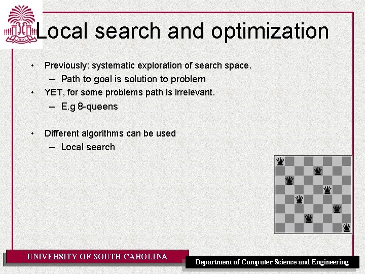
Local search and optimization • Previously: systematic exploration of search space. – Path to goal is solution to problem • YET, for some problems path is irrelevant. – E. g 8 -queens • Different algorithms can be used – Local search UNIVERSITY OF SOUTH CAROLINA Department of Computer Science and Engineering

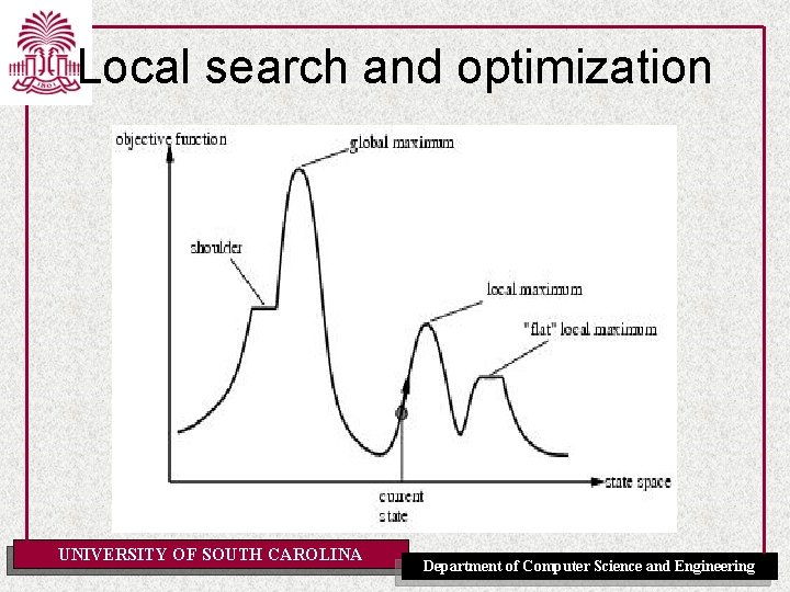
Local search and optimization • • Local search= use single current state and move to neighboring states. Advantages: – Use very little memory – Find often reasonable solutions in large or infinite state spaces. • Are also useful for pure optimization problems. – Find best state according to some objective function. – e. g. survival of the fittest as a metaphor for optimization. UNIVERSITY OF SOUTH CAROLINA Department of Computer Science and Engineering

Local search and optimization UNIVERSITY OF SOUTH CAROLINA Department of Computer Science and Engineering

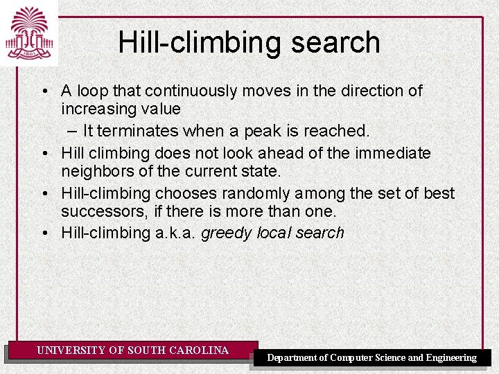
Hill-climbing search • A loop that continuously moves in the direction of increasing value – It terminates when a peak is reached. • Hill climbing does not look ahead of the immediate neighbors of the current state. • Hill-climbing chooses randomly among the set of best successors, if there is more than one. • Hill-climbing a. k. a. greedy local search UNIVERSITY OF SOUTH CAROLINA Department of Computer Science and Engineering

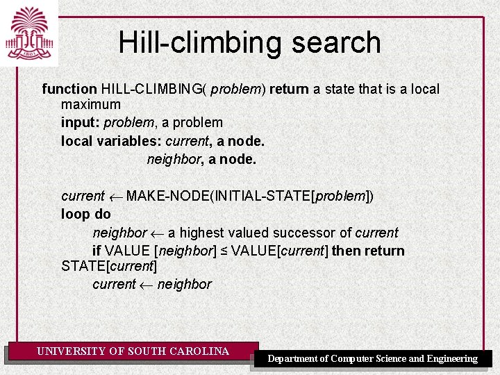
Hill-climbing search function HILL-CLIMBING( problem) return a state that is a local maximum input: problem, a problem local variables: current, a node. neighbor, a node. current MAKE-NODE(INITIAL-STATE[problem]) loop do neighbor a highest valued successor of current if VALUE [neighbor] ≤ VALUE[current] then return STATE[current] current neighbor UNIVERSITY OF SOUTH CAROLINA Department of Computer Science and Engineering

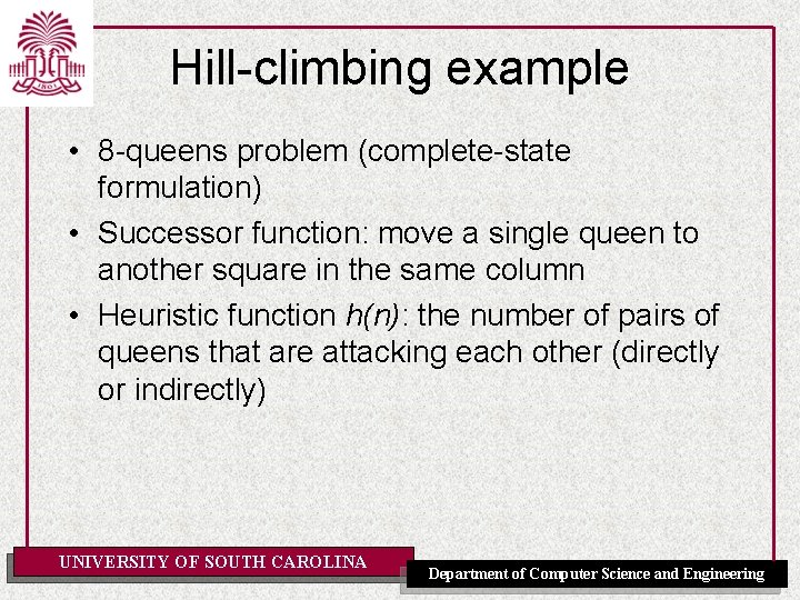
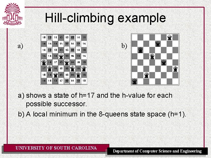
Hill-climbing example • 8 -queens problem (complete-state formulation) • Successor function: move a single queen to another square in the same column • Heuristic function h(n): the number of pairs of queens that are attacking each other (directly or indirectly) UNIVERSITY OF SOUTH CAROLINA Department of Computer Science and Engineering

Hill-climbing example a) b) a) shows a state of h=17 and the h-value for each possible successor. b) A local minimum in the 8 -queens state space (h=1). UNIVERSITY OF SOUTH CAROLINA Department of Computer Science and Engineering

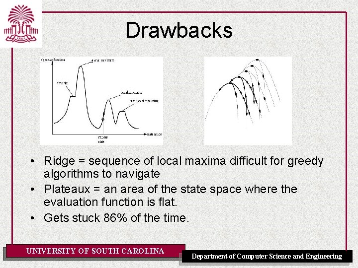
Drawbacks • Ridge = sequence of local maxima difficult for greedy algorithms to navigate • Plateaux = an area of the state space where the evaluation function is flat. • Gets stuck 86% of the time. UNIVERSITY OF SOUTH CAROLINA Department of Computer Science and Engineering

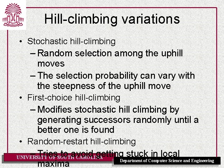
Hill-climbing variations • Stochastic hill-climbing – Random selection among the uphill moves – The selection probability can vary with the steepness of the uphill move • First-choice hill-climbing – Modifies stochastic hill climbing by generating successors randomly until a better one is found • Random-restart hill-climbing – Tries to avoid getting stuck in local Department of Computer Science and Engineering maxima UNIVERSITY OF SOUTH CAROLINA

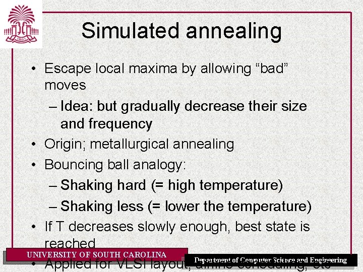
Simulated annealing • Escape local maxima by allowing “bad” moves – Idea: but gradually decrease their size and frequency • Origin; metallurgical annealing • Bouncing ball analogy: – Shaking hard (= high temperature) – Shaking less (= lower the temperature) • If T decreases slowly enough, best state is reached UNIVERSITY OF SOUTH CAROLINA Computer Science and Engineering • Applied for VLSI layout, Department airlineofscheduling, etc

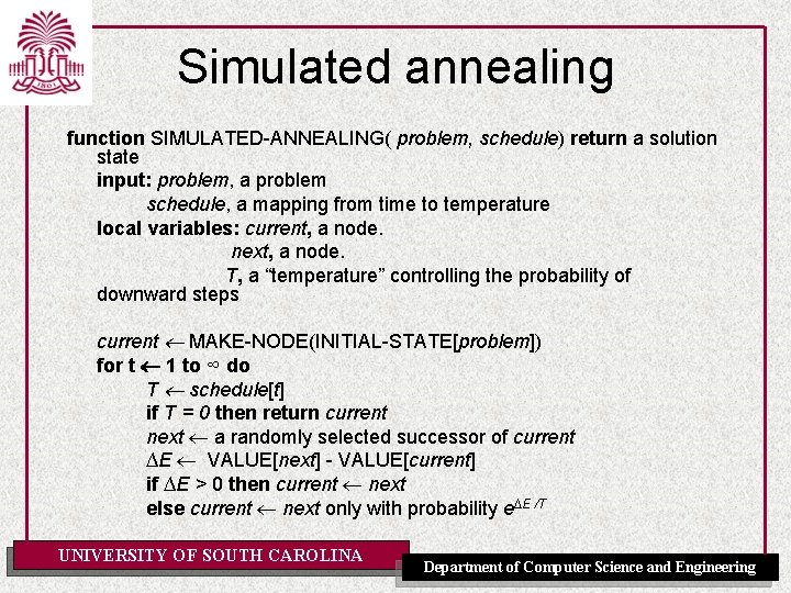
Simulated annealing function SIMULATED-ANNEALING( problem, schedule) return a solution state input: problem, a problem schedule, a mapping from time to temperature local variables: current, a node. next, a node. T, a “temperature” controlling the probability of downward steps current MAKE-NODE(INITIAL-STATE[problem]) for t 1 to ∞ do T schedule[t] if T = 0 then return current next a randomly selected successor of current ∆E VALUE[next] - VALUE[current] if ∆E > 0 then current next else current next only with probability e∆E /T UNIVERSITY OF SOUTH CAROLINA Department of Computer Science and Engineering

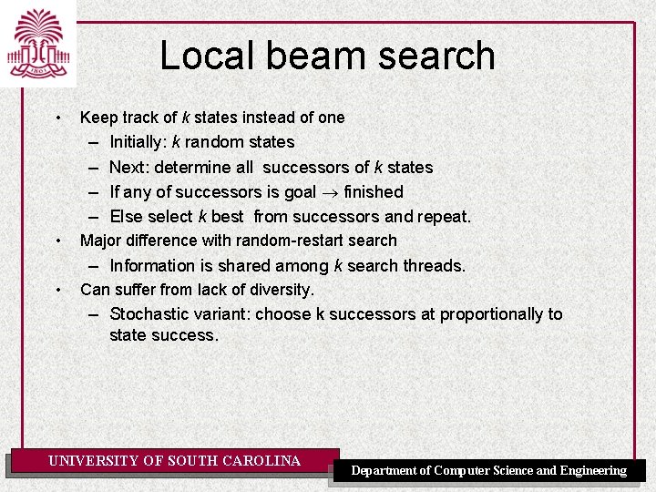
Local beam search • Keep track of k states instead of one – – • Initially: k random states Next: determine all successors of k states If any of successors is goal finished Else select k best from successors and repeat. Major difference with random-restart search – Information is shared among k search threads. • Can suffer from lack of diversity. – Stochastic variant: choose k successors at proportionally to state success. UNIVERSITY OF SOUTH CAROLINA Department of Computer Science and Engineering

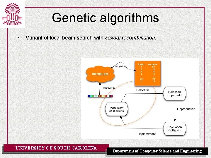
Genetic algorithms • Variant of local beam search with sexual recombination. UNIVERSITY OF SOUTH CAROLINA Department of Computer Science and Engineering

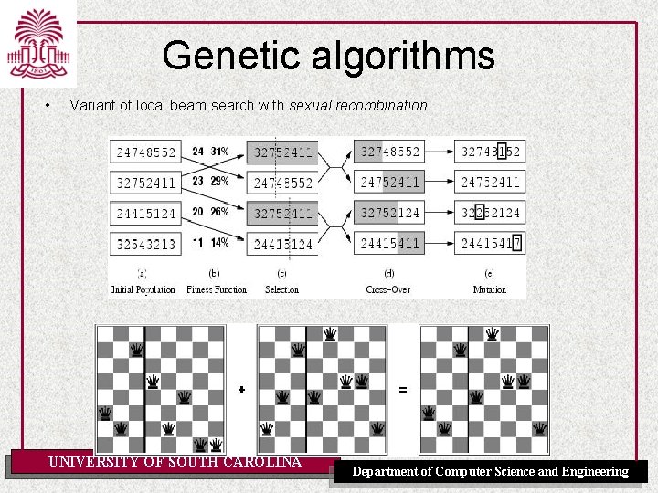
Genetic algorithms • Variant of local beam search with sexual recombination. UNIVERSITY OF SOUTH CAROLINA Department of Computer Science and Engineering

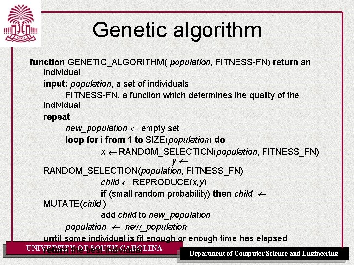
Genetic algorithm function GENETIC_ALGORITHM( population, FITNESS-FN) return an individual input: population, a set of individuals FITNESS-FN, a function which determines the quality of the individual repeat new_population empty set loop for i from 1 to SIZE(population) do x RANDOM_SELECTION(population, FITNESS_FN) y RANDOM_SELECTION(population, FITNESS_FN) child REPRODUCE(x, y) if (small random probability) then child MUTATE(child ) add child to new_population until some individual is fit enough or enough time has elapsed UNIVERSITY OFbest SOUTH CAROLINA return the individual Department of Computer Science and Engineering

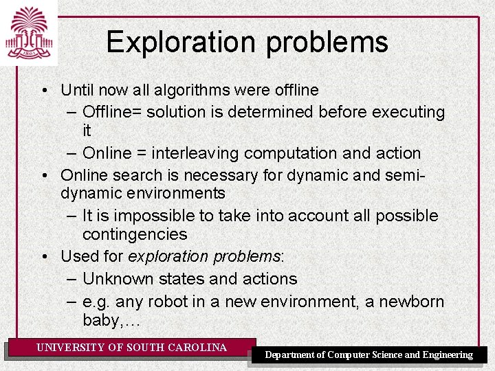
Exploration problems • Until now all algorithms were offline – Offline= solution is determined before executing it – Online = interleaving computation and action • Online search is necessary for dynamic and semidynamic environments – It is impossible to take into account all possible contingencies • Used for exploration problems: – Unknown states and actions – e. g. any robot in a new environment, a newborn baby, … UNIVERSITY OF SOUTH CAROLINA Department of Computer Science and Engineering

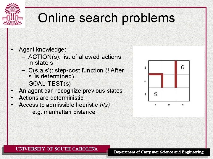
Online search problems • Agent knowledge: – ACTION(s): list of allowed actions in state s – C(s, a, s’): step-cost function (! After s’ is determined) – GOAL-TEST(s) • An agent can recognize previous states • Actions are deterministic • Access to admissible heuristic h(s) e. g. manhattan distance UNIVERSITY OF SOUTH CAROLINA Department of Computer Science and Engineering

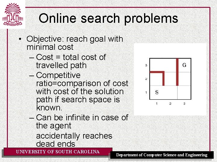
Online search problems • Objective: reach goal with minimal cost – Cost = total cost of travelled path – Competitive ratio=comparison of cost with cost of the solution path if search space is known. – Can be infinite in case of the agent accidentally reaches dead ends UNIVERSITY OF SOUTH CAROLINA Department of Computer Science and Engineering

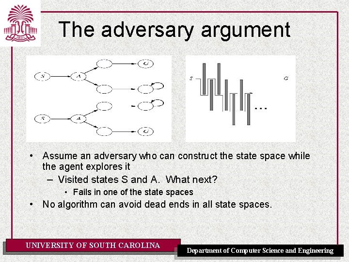
The adversary argument • Assume an adversary who can construct the state space while the agent explores it – Visited states S and A. What next? • Fails in one of the state spaces • No algorithm can avoid dead ends in all state spaces. UNIVERSITY OF SOUTH CAROLINA Department of Computer Science and Engineering

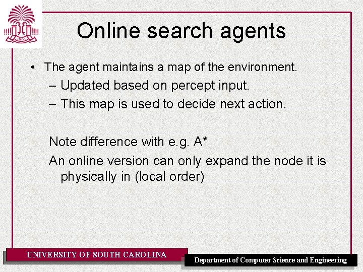
Online search agents • The agent maintains a map of the environment. – Updated based on percept input. – This map is used to decide next action. Note difference with e. g. A* An online version can only expand the node it is physically in (local order) UNIVERSITY OF SOUTH CAROLINA Department of Computer Science and Engineering

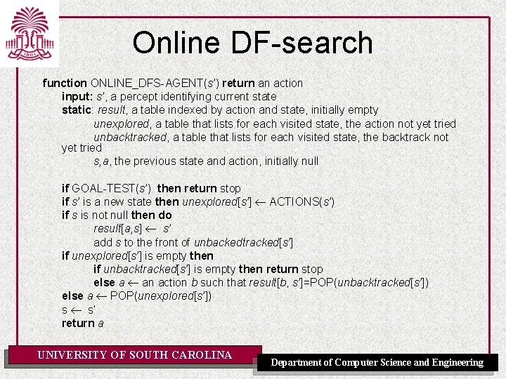
Online DF-search function ONLINE_DFS-AGENT(s’) return an action input: s’, a percept identifying current state static: result, a table indexed by action and state, initially empty unexplored, a table that lists for each visited state, the action not yet tried unbacktracked, a table that lists for each visited state, the backtrack not yet tried s, a, the previous state and action, initially null if GOAL-TEST(s’) then return stop if s’ is a new state then unexplored[s’] ACTIONS(s’) if s is not null then do result[a, s] s’ add s to the front of unbackedtracked[s’] if unexplored[s’] is empty then if unbacktracked[s’] is empty then return stop else a an action b such that result[b, s’]=POP(unbacktracked[s’]) else a POP(unexplored[s’]) s s’ return a UNIVERSITY OF SOUTH CAROLINA Department of Computer Science and Engineering

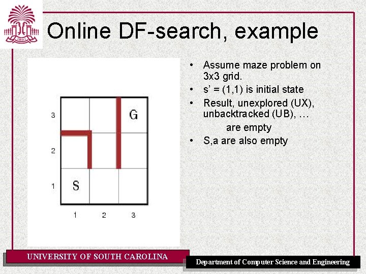
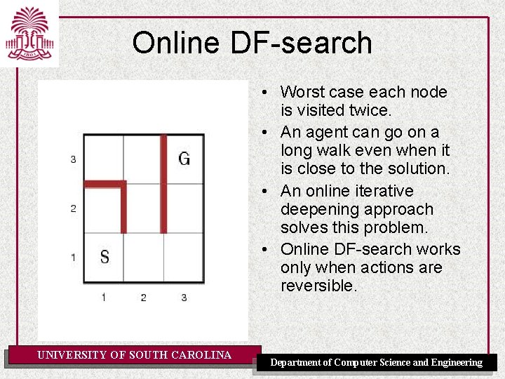
Online DF-search, example • Assume maze problem on 3 x 3 grid. • s’ = (1, 1) is initial state • Result, unexplored (UX), unbacktracked (UB), … are empty • S, a are also empty UNIVERSITY OF SOUTH CAROLINA Department of Computer Science and Engineering

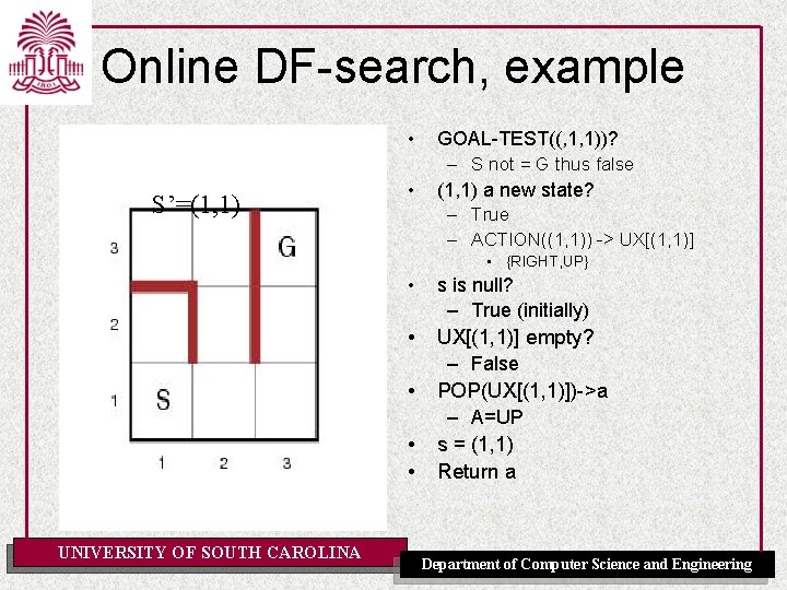
Online DF-search, example • S’=(1, 1) • GOAL-TEST((, 1, 1))? – S not = G thus false (1, 1) a new state? – True – ACTION((1, 1)) -> UX[(1, 1)] • {RIGHT, UP} • s is null? – True (initially) • UX[(1, 1)] empty? – False POP(UX[(1, 1)])->a – A=UP s = (1, 1) Return a • • • UNIVERSITY OF SOUTH CAROLINA Department of Computer Science and Engineering

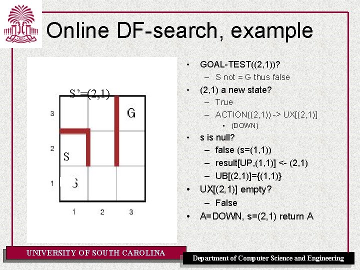
Online DF-search, example • S’=(2, 1) • GOAL-TEST((2, 1))? – S not = G thus false (2, 1) a new state? – True – ACTION((2, 1)) -> UX[(2, 1)] • {DOWN} • s is null? – false (s=(1, 1)) – result[UP, (1, 1)] <- (2, 1) – UB[(2, 1)]={(1, 1)} • UX[(2, 1)] empty? – False A=DOWN, s=(2, 1) return A S • UNIVERSITY OF SOUTH CAROLINA Department of Computer Science and Engineering

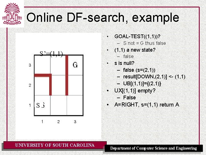
Online DF-search, example • S’=(1, 1) • • • S UNIVERSITY OF SOUTH CAROLINA • GOAL-TEST((1, 1))? – S not = G thus false (1, 1) a new state? – false s is null? – false (s=(2, 1)) – result[DOWN, (2, 1)] <- (1, 1) – UB[(1, 1)]={(2, 1)} UX[(1, 1)] empty? – False A=RIGHT, s=(1, 1) return A Department of Computer Science and Engineering

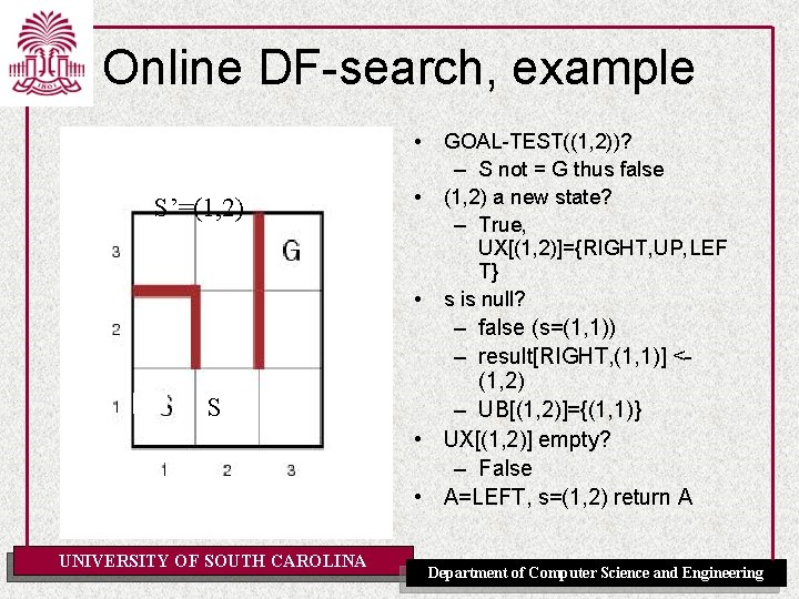
Online DF-search, example • S’=(1, 2) • • S UNIVERSITY OF SOUTH CAROLINA GOAL-TEST((1, 2))? – S not = G thus false (1, 2) a new state? – True, UX[(1, 2)]={RIGHT, UP, LEF T} s is null? – false (s=(1, 1)) – result[RIGHT, (1, 1)] <(1, 2) – UB[(1, 2)]={(1, 1)} • UX[(1, 2)] empty? – False • A=LEFT, s=(1, 2) return A Department of Computer Science and Engineering

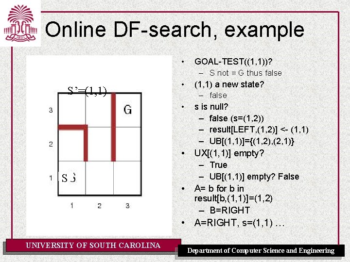
Online DF-search, example • S’=(1, 1) • • • S • GOAL-TEST((1, 1))? – S not = G thus false (1, 1) a new state? – false s is null? – false (s=(1, 2)) – result[LEFT, (1, 2)] <- (1, 1) – UB[(1, 1)]={(1, 2), (2, 1)} UX[(1, 1)] empty? – True – UB[(1, 1)] empty? False A= b for b in result[b, (1, 1)]=(1, 2) – B=RIGHT • A=RIGHT, s=(1, 1) … UNIVERSITY OF SOUTH CAROLINA Department of Computer Science and Engineering

Online DF-search • Worst case each node is visited twice. • An agent can go on a long walk even when it is close to the solution. • An online iterative deepening approach solves this problem. • Online DF-search works only when actions are reversible. UNIVERSITY OF SOUTH CAROLINA Department of Computer Science and Engineering

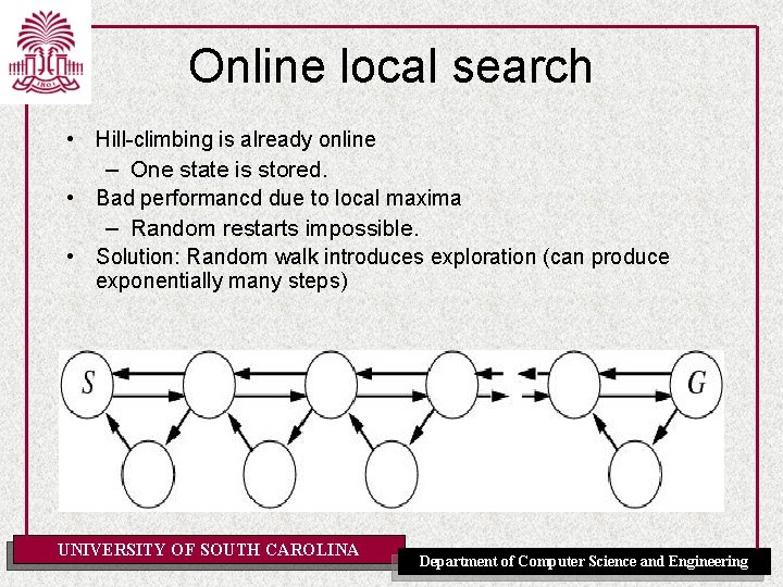
Online local search • Hill-climbing is already online – One state is stored. • Bad performancd due to local maxima – Random restarts impossible. • Solution: Random walk introduces exploration (can produce exponentially many steps) UNIVERSITY OF SOUTH CAROLINA Department of Computer Science and Engineering

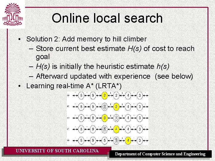
Online local search • Solution 2: Add memory to hill climber – Store current best estimate H(s) of cost to reach goal – H(s) is initially the heuristic estimate h(s) – Afterward updated with experience (see below) • Learning real-time A* (LRTA*) UNIVERSITY OF SOUTH CAROLINA Department of Computer Science and Engineering

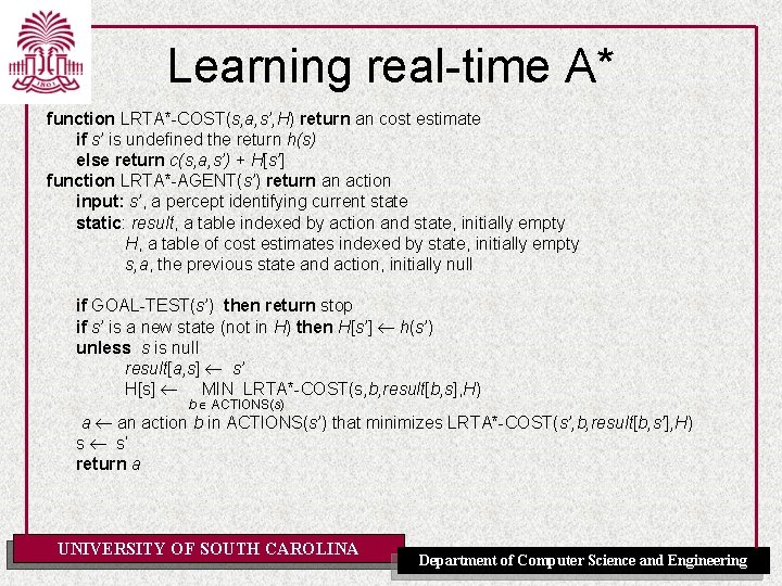
Learning real-time A* function LRTA*-COST(s, a, s’, H) return an cost estimate if s’ is undefined the return h(s) else return c(s, a, s’) + H[s’] function LRTA*-AGENT(s’) return an action input: s’, a percept identifying current state static: result, a table indexed by action and state, initially empty H, a table of cost estimates indexed by state, initially empty s, a, the previous state and action, initially null if GOAL-TEST(s’) then return stop if s’ is a new state (not in H) then H[s’] h(s’) unless s is null result[a, s] s’ H[s] MIN LRTA*-COST(s, b, result[b, s], H) b ACTIONS(s) a an action b in ACTIONS(s’) that minimizes LRTA*-COST(s’, b, result[b, s’], H) s s’ return a UNIVERSITY OF SOUTH CAROLINA Department of Computer Science and Engineering