CSC 589 Introduction to Computer Vision Lecture 6

CSC 589 Introduction to Computer Vision Lecture 6 Image Derivative, Image-Denoising Bei Xiao

Last lecture • Linear Algebra • Matrix computation in Python

Today’s lecture • • • More on Image derivatives Quiz Image De-noising Median Filter Introduction to Frequency analysis • Homework is due today! Please follow hand-in instructions. Be sure to include your write-up document!!

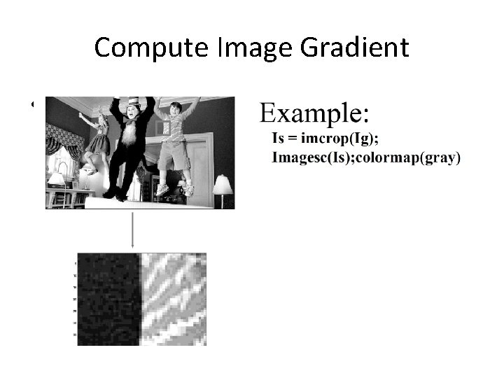
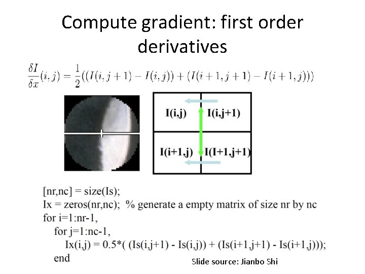
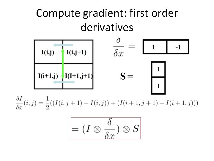
Compute Image Gradient • The first order derivative of Image I in x, and in y direction

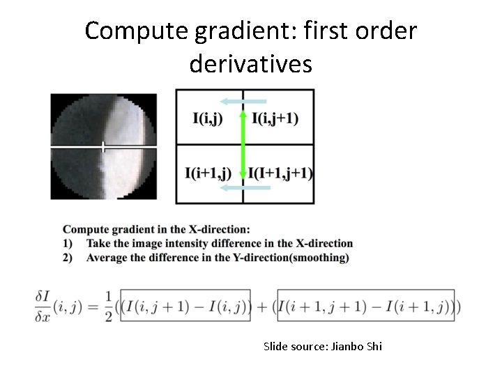
Compute gradient: first order derivatives Slide source: Jianbo Shi

Compute gradient: first order derivatives Slide source: Jianbo Shi

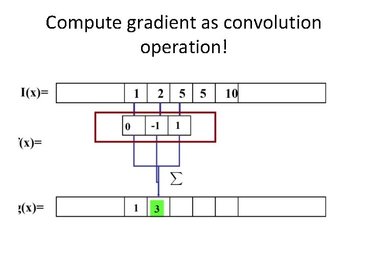
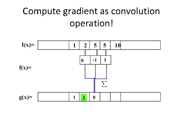
Compute gradient as convolution operation!

Compute gradient as convolution operation!

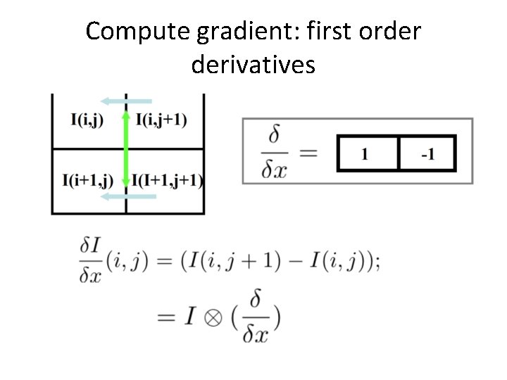
Compute gradient: first order derivatives

Compute gradient: first order derivatives

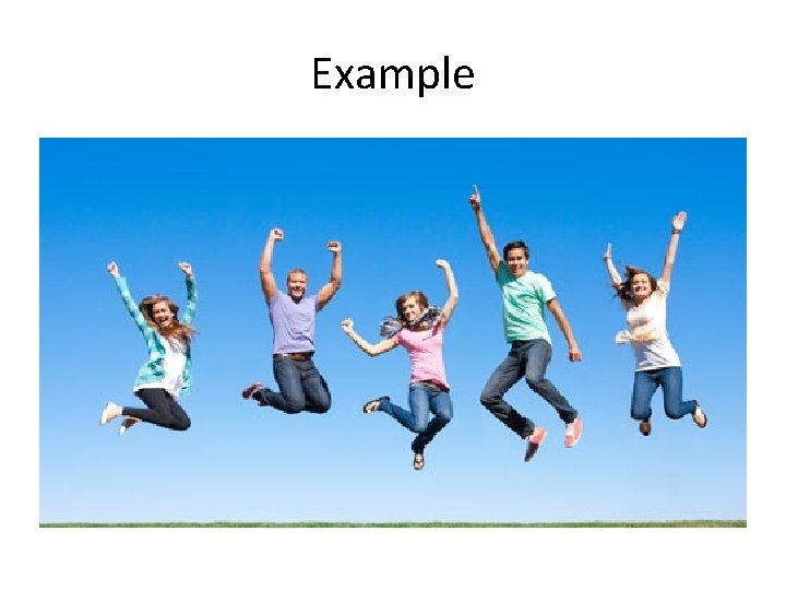
Example

Usage in Python • • • s 1 = np. array([1, 1]) dx = np. array([1, -1]) dy = np. array([1, -1]) x = ndimage. convolve 1 d(l, dx, axis= 0) gx_I = ndimage. convolve(x, s)

Usage in Python • • • s 1 = np. array([1, 1]) dx = np. array([1, -1]) dy = np. array([1, -1]) y = ndimage. convolve 1 d(l, dx, axis= 1) gy_I = ndimage. convolve(y, s) Or : gx_I, gy_I = np. gradient(l)[: 2]

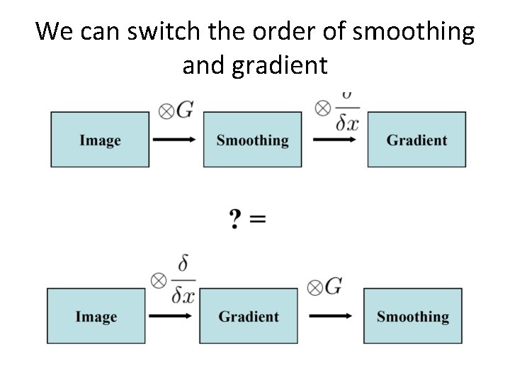
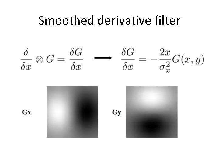
We can switch the order of smoothing and gradient

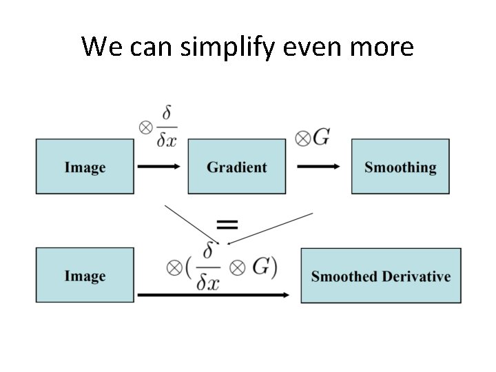
We can simplify even more

Smoothed derivative filter

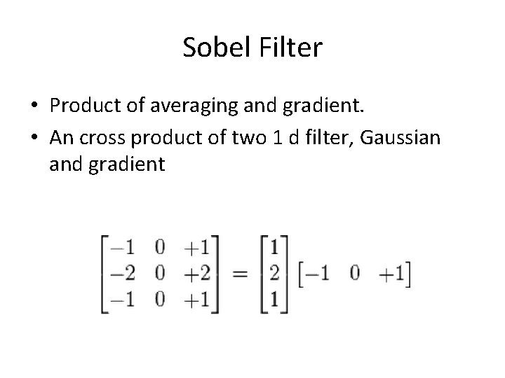
Sobel Filter • Product of averaging and gradient. • An cross product of two 1 d filter, Gaussian and gradient

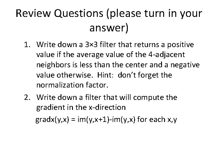
Review Questions (please turn in your answer) 1. Write down a 3× 3 filter that returns a positive value if the average value of the 4 -adjacent neighbors is less than the center and a negative value otherwise. Hint: don’t forget the normalization factor. 2. Write down a filter that will compute the gradient in the x-direction gradx(y, x) = im(y, x+1)-im(y, x) for each x, y

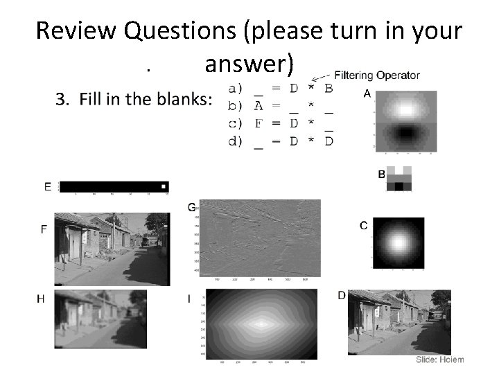
Review Questions (please turn in your answer)

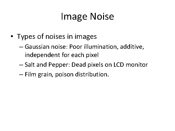
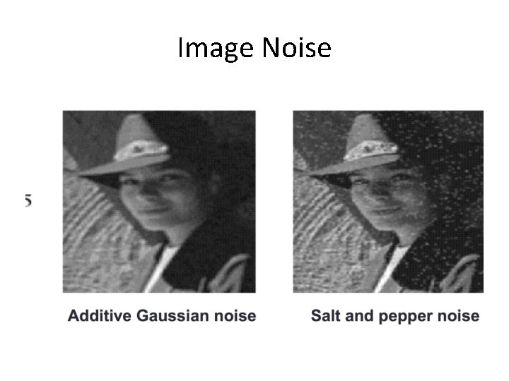
Image Noise • Types of noises in images – Gaussian noise: Poor illumination, additive, independent for each pixel – Salt and Pepper: Dead pixels on LCD monitor – Film grain, poison distribution.

Image Noise

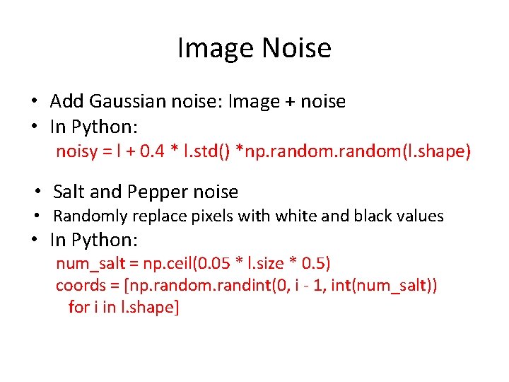
Image Noise • Add Gaussian noise: Image + noise • In Python: noisy = l + 0. 4 * l. std() *np. random(l. shape) • Salt and Pepper noise • Randomly replace pixels with white and black values • In Python: num_salt = np. ceil(0. 05 * l. size * 0. 5) coords = [np. random. randint(0, i - 1, int(num_salt)) for i in l. shape]

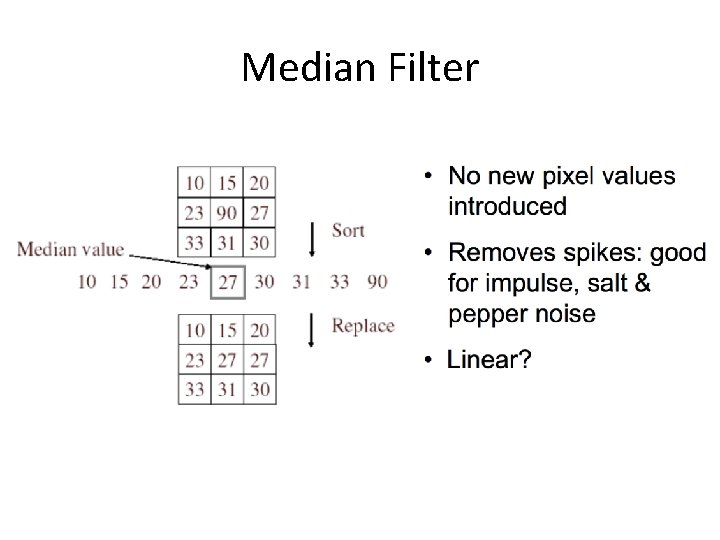
Median Filter X = [2 80 6 3] The median filter has a window size 3 The median filtered out signal y will be: Y[1] = Median [2 2 80] = 2 Y[2] = Median [2 80 6] = 6 Y[3] = Median[80 6 3] = 6 Y[3] = Median [6 3 3 ] = 3 Notice the repeating of the first element Selecting one pixel as a time; Not as efficient as Gaussian Filter

Median Filter

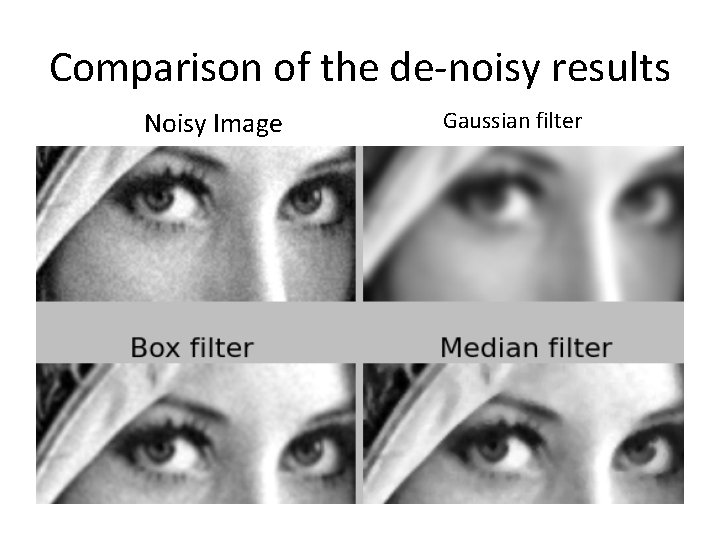
Comparison of the de-noisy results Noisy Image Gaussian filter

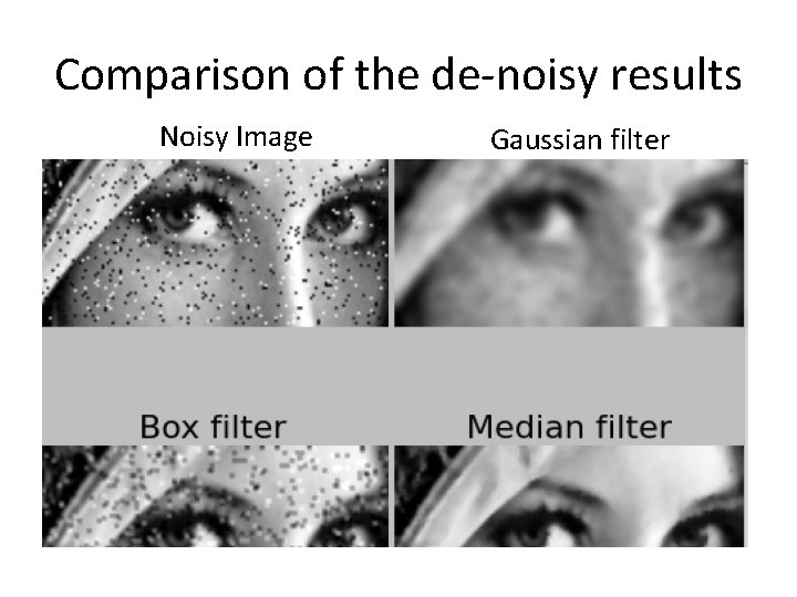
Comparison of the de-noisy results Noisy Image Gaussian filter

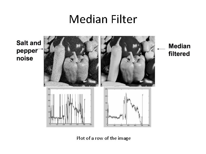
Median Filter Plot of a row of the image

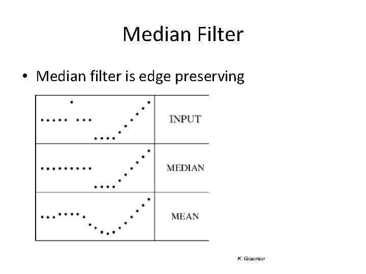
Median Filter • Median filter is edge preserving

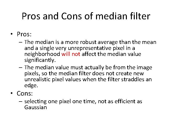
Pros and Cons of median filter • Pros: – The median is a more robust average than the mean and a single very unrepresentative pixel in a neighborhood will not affect the median value significantly. – The median value must actually be from the image pixels, so the median filter does not create new unrealistic pixel values when the filter straddles an edge. • Cons: – selecting one pixel one time, not as efficient as Gaussian

Median Filter in Pyton • med_denoised = ndimage. median_filter(noisy, windowsize)

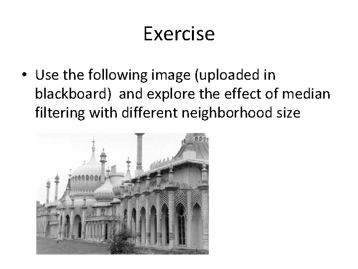
Exercise • Use the following image (uploaded in blackboard) and explore the effect of median filtering with different neighborhood size

Exercise • Unlike Gaussian filter, median filter is nonlinear. • Median [A(x) + B(x)] = median[A(x)] + median[B(x)] • Illustrate this to yourself by performing smoothing and pixel addition (in the order above) to a set of test images

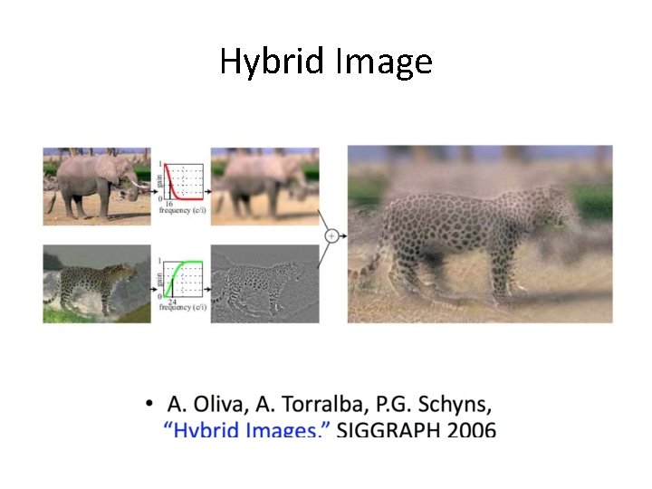
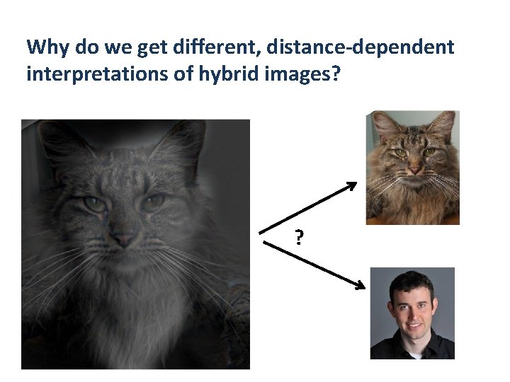
Hybrid Image

Why do we get different, distance-dependent interpretations of hybrid images? ?

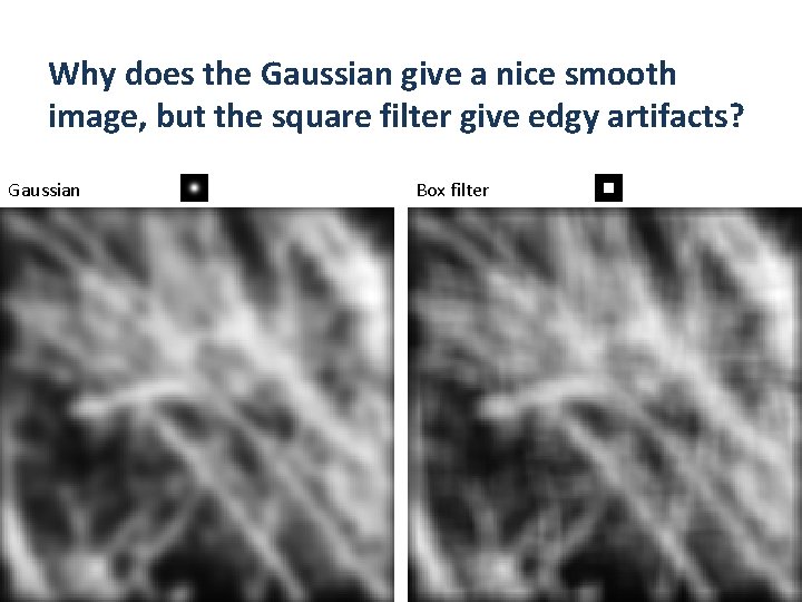
Why does the Gaussian give a nice smooth image, but the square filter give edgy artifacts? Gaussian Box filter