CSc 553 Principles of Compilation 05 Program Analysis

CSc 553 Principles of Compilation 05. Program Analysis Saumya Debray The University of Arizona Tucson, AZ 85721

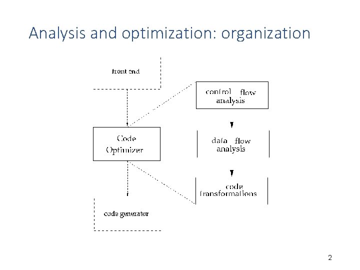
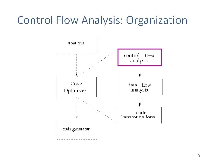
Analysis and optimization: organization 2

CONTROL FLOW ANALYSIS 3

Goals To obtain higher-level information about the possible control flow behaviors of the program, e. g. : − “which blocks are guaranteed to have been executed if control reaches some block B? ” − “which blocks are guaranteed to be executed once control reaches some block B? ” − “what is the loop structure of the code? ” Criteria: − must be “safe, ” i. e. , must take into account all possible executions of the program 4

Control Flow Analysis: Organization 5

Dominators 6

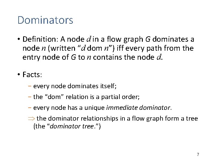
Dominators • Definition: A node d in a flow graph G dominates a node n (written “d dom n”) iff every path from the entry node of G to n contains the node d. • Facts: − every node dominates itself; − the “dom” relation is a partial order; − every node has a unique immediate dominator. the dominator relationships in a flow graph form a tree (the “dominator tree. ”) 7

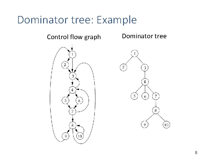
Dominator tree: Example Control flow graph Dominator tree 8

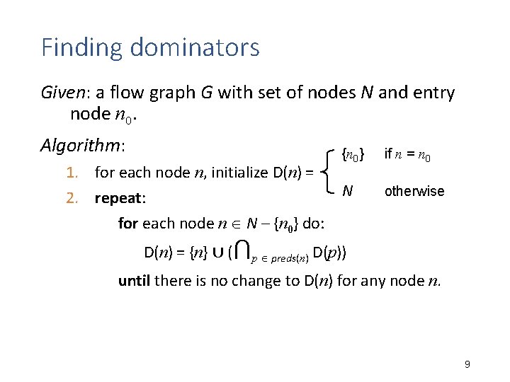
Finding dominators Given: a flow graph G with set of nodes N and entry node n 0. Algorithm: {n 0} 1. for each node n, initialize D(n) = N 2. repeat: for each node n N – {n 0} do: if n = n 0 otherwise D(n) = {n} ∪ (⋂p preds(n) D(p)) until there is no change to D(n) for any node n. 9

Natural loops 10

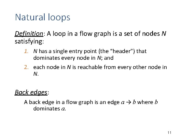
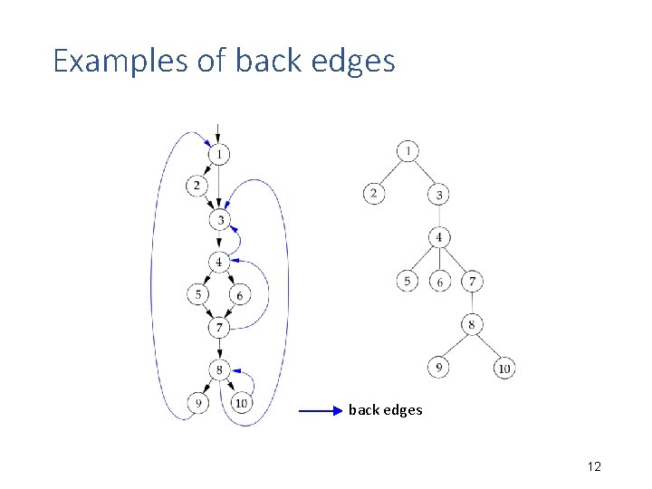
Natural loops Definition: A loop in a flow graph is a set of nodes N satisfying: 1. N has a single entry point (the “header”) that dominates every node in N; and 2. each node in N is reachable from every other node in N. Back edges: A back edge in a flow graph is an edge a → b where b dominates a. 11

Examples of back edges 12

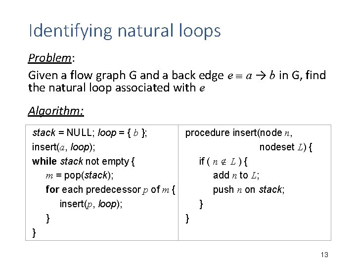
Identifying natural loops Problem: Given a flow graph G and a back edge e a → b in G, find the natural loop associated with e Algorithm: stack = NULL; loop = { b }; insert(a, loop); while stack not empty { m = pop(stack); for each predecessor p of m { insert(p, loop); } } procedure insert(node n, nodeset L) { if ( n L ) { add n to L; push n on stack; } } 13

DATA FLOW ANALYSIS 14

Dataflow analysis: goals • To infer invariants about the runtime behavior of programs − “what must be true, for any possible execution, whenever control reaches this point in the code? ” − this information is then used for various purposes, e. g. , optimizing transformations, security analyses, . . . • Criteria: − must be “safe, ” i. e. , must take into account all possible executions of the program. 15

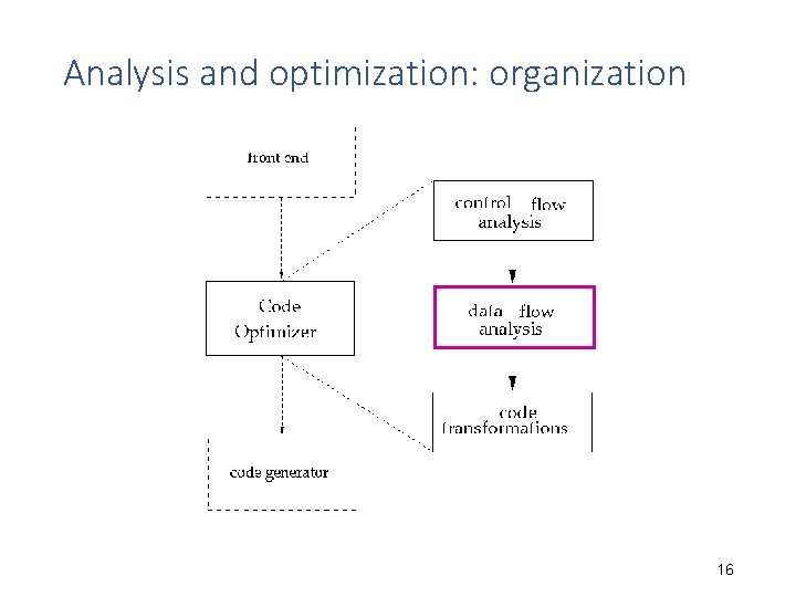
Analysis and optimization: organization 16

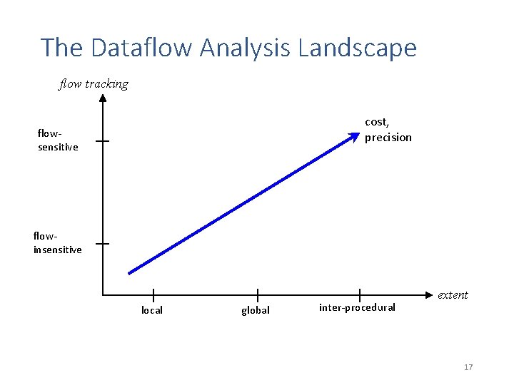
The Dataflow Analysis Landscape flow tracking cost, precision flowsensitive flowinsensitive local global inter-procedural extent 17

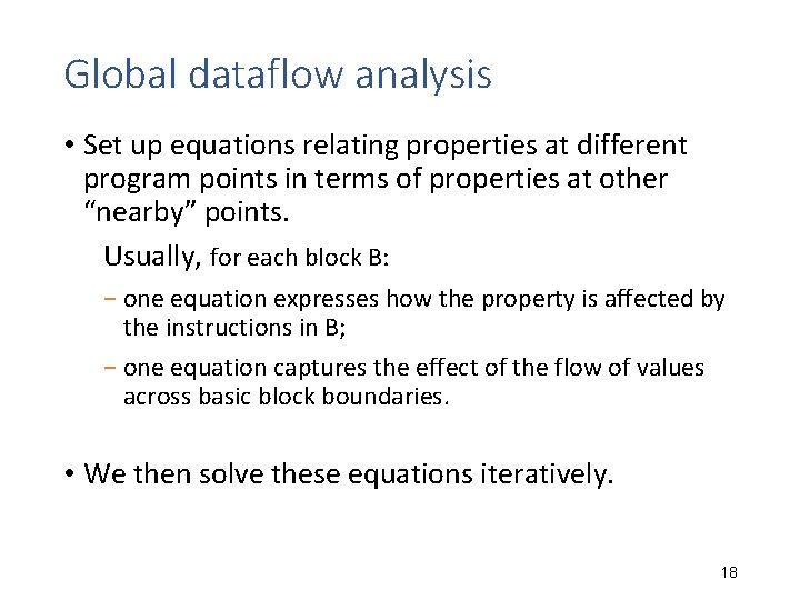
Global dataflow analysis • Set up equations relating properties at different program points in terms of properties at other “nearby” points. Usually, for each block B: − one equation expresses how the property is affected by the instructions in B; − one equation captures the effect of the flow of values across basic block boundaries. • We then solve these equations iteratively. 18

Analysis 1 Reaching definitions 19

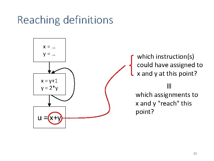
Reaching definitions x=… y=… u = x+y x = y+1 y = 2*y which instruction(s) could have assigned to x and y at this point? which assignments to x and y "reach" this point? 20

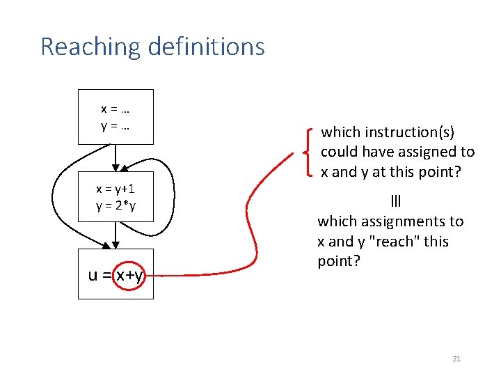
Reaching definitions x=… y=… u = x+y x = y+1 y = 2*y which instruction(s) could have assigned to x and y at this point? which assignments to x and y "reach" this point? 21

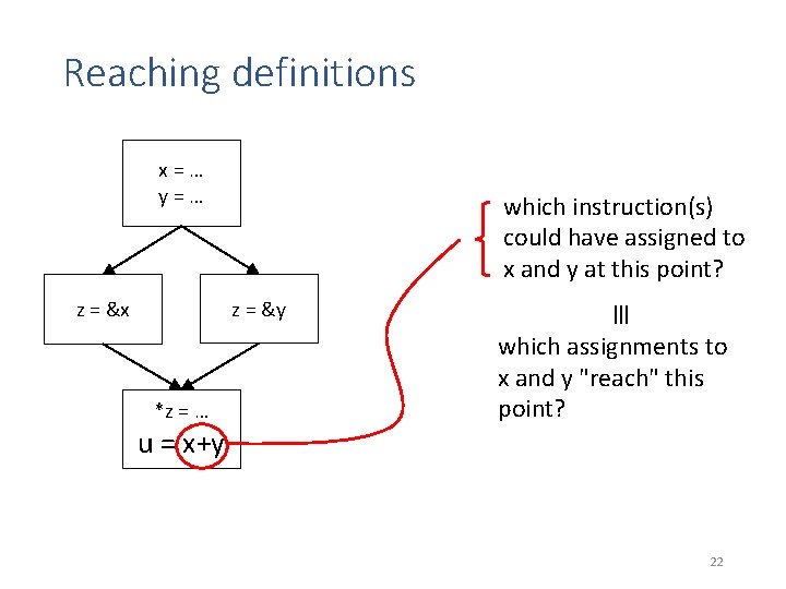
Reaching definitions x=… y=… which instruction(s) could have assigned to x and y at this point? *z = … u = x+y z = &x which assignments to x and y "reach" this point? 22

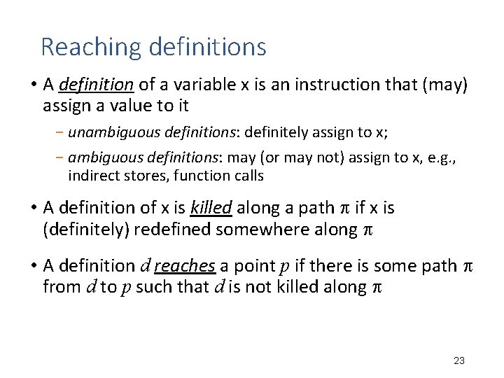
Reaching definitions • A definition of a variable x is an instruction that (may) assign a value to it − unambiguous definitions: definitely assign to x; − ambiguous definitions: may (or may not) assign to x, e. g. , indirect stores, function calls • A definition of x is killed along a path if x is (definitely) redefined somewhere along • A definition d reaches a point p if there is some path from d to p such that d is not killed along 23

Computing reaching definitions in[B] : definitions reaching B's entry gen[B] : definitions in B that reach the end of B kill[B] : definitions that are killed by definitions in B Idea: express out[B] in terms of in[B] B a basic block out[B] : definitions reaching B's exit express how the code in B transforms in[B] to out[B] − gen[B]: definitions added to in[B] − kill[B]: definitions removed from in[B] 24

Reaching definitions: dataflow equations out[B] = gen[B] (in[B] – kill[B]) in[B] = { out[X] | X is a predecessor of B} gen[B]: the set of definitions in B that reach the end of B kill[B]: the set of definitions (in the entire function) that are killed by definitions within B in[B]: the set of definitions that reach the entry to B out[B]: the set of definitions that reach the exit from B 25

Reaching definitions: dataflow equations out[B] = gen[B] (in[B] – kill[B]) in[B] = { out[X] | X is a predecessor of B} • Points to note: − out[B] is computed from in[B] computed from predecessors of B o information is propagated along direction of control flow o "forward dataflow analysis" − in the presence of loops, the equations become circular 26

Reaching definitions: gen and kill sets For each block B: gen[B], kill[B] computed once, at the beginning, using information local to B: 1. . G = K = ; 2. for each instruction I in B, going forward, do: o let I ‘x = …’, and Dx = {J | J is an instruction defining x}; o G = (G – Dx) { I } o K = (K Dx) – { I } 3. gen[B] = G at the end of B; kill[B] = K at the end of B; 27

Solving dataflow equations • Choose an initial approximation for in[B], out[B]. • Iteratively improve these approximations: − let ini[B], outi[B] be values obtained after iteration i. − recompute dataflow equations using these values: outi+1[B] = gen[B] ⋃ (ini[B] – kill[B]) ini+1[B] = ⋃ { outi[X] | X is a predecessor of B} until the equations converge, i. e. , there is no change to in[B] or out[B] for any B. 28

Solving dataflow equations for each block B, set out[B] = gen[B]; /* assumes in[B] = */ chg = true while ( chg ) { chg = false for each block B { in[B] = ⋃ { out[X] | X a predecessor of B }; oldout = out[B]; out[B] = gen[B] ⋃ (in[B] – kill[B]); if (out[B] oldout) chg = true; } } 29

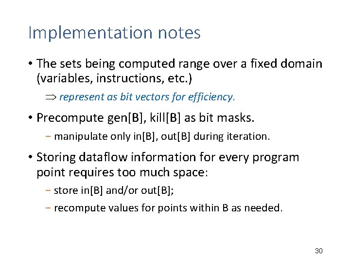
Implementation notes • The sets being computed range over a fixed domain (variables, instructions, etc. ) represent as bit vectors for efficiency. • Precompute gen[B], kill[B] as bit masks. − manipulate only in[B], out[B] during iteration. • Storing dataflow information for every program point requires too much space: − store in[B] and/or out[B]; − recompute values for points within B as needed. 30

Analysis 2 Liveness analysis 31

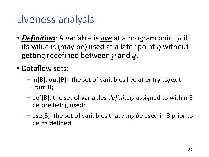
Liveness analysis • Definition: A variable is live at a program point p if its value is (may be) used at a later point q without getting redefined between p and q. • Dataflow sets: − in[B], out[B] : the set of variables live at entry to/exit from B; − def[B]: the set of variables definitely assigned to within B before being used; − use[B]: the set of variables that may be used in B prior to being defined. 32

Liveness analysis: def and use sets For each block B: def[B], use[B] are computed once, at the beginning, using information local to B: 1. D = U = ; 2. for each instruction I in B, going backward from the end, do: /* compute D, U immediately before I */ o let I ‘x = y z’; o D = (D { x }) – { y, z }; o U = (U – { x }) { y, z }; 3. def[B] = D at the beginning of B; use[B] = U at the beginning of B. 33

Liveness analysis: equations and algorithm in[B] = use[B] (out[B] – def[B]) out[B] = { in[X] | X is a successor of B }. Algorithm: 1. for each basic block B, set in[B] = use[B]; 2. repeat for each basic block B { out[B] = { in[X] | X is a successor of B }; in[B] = use[B] (out[B] – def[B]); } until no change to in[B], out[B] for any B. 34

Analysis 3 Available expressions 35

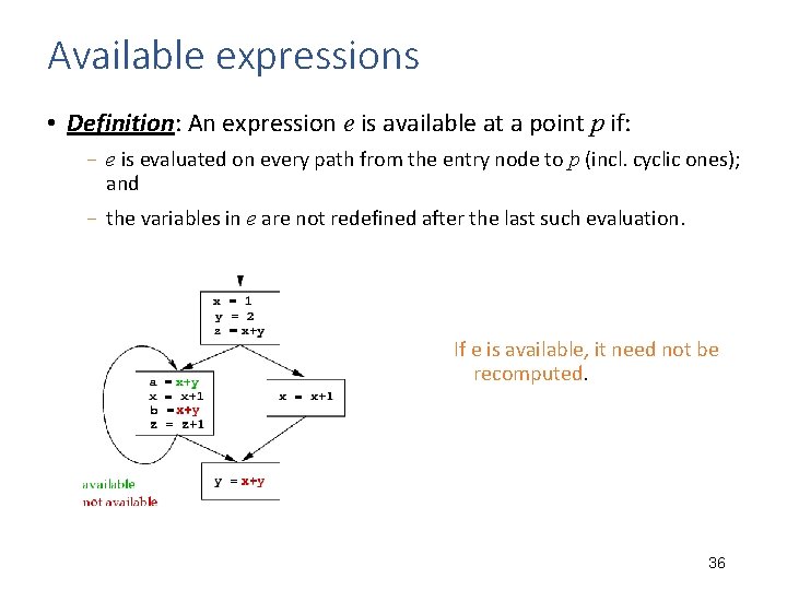
Available expressions • Definition: An expression e is available at a point p if: − e is evaluated on every path from the entry node to p (incl. cyclic ones); and − the variables in e are not redefined after the last such evaluation. If e is available, it need not be recomputed. 36

Available expressions: dataflow equations • in[B], out[B]: sets of expressions available at B’s entry/exit. • gen[B]: the set of expressions e that are evaluated in B, s. t. no variable in e is redefined after the last evaluation of e in B. • kill[B]: the set of expressions e in the program (function) s. t. B may redefine some variables in e without subsequently evaluating e. in[B 0] = (B 0 is the entry node) in[B] = { out[X] | X a predecessor of B} if B B 0 out[B] = gen[B] (in[B] – kill[B]) 37

Available expressions: gen and kill sets For each block B: gen[B], kill[B] computed once, at the beginning of the analysis, using information local to B: 1. G = K = ; 2. for each instruction I in B, going forward, do: o let I ‘x = y z’, and Ex = all expressions involving x; o G = (G { ‘y z’ }) – Ex; o K = (K – { ‘y z’ }) Ex; 3. gen[B] = G at the end of B; kill[B] = K at the end of B; 38

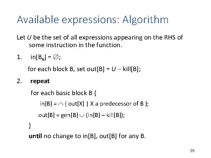
Available expressions: Algorithm Let U be the set of all expressions appearing on the RHS of some instruction in the function. 1. in[B 0] = ; for each block B, set out[B] = U – kill[B]; 2. repeat for each basic block B { in[B] = { out[X] | X a predecessor of B }; out[B] = gen[B] (in[B] – kill[B]); } until no change to in[B], out[B] for any B. 39

Comparing different analyses 40

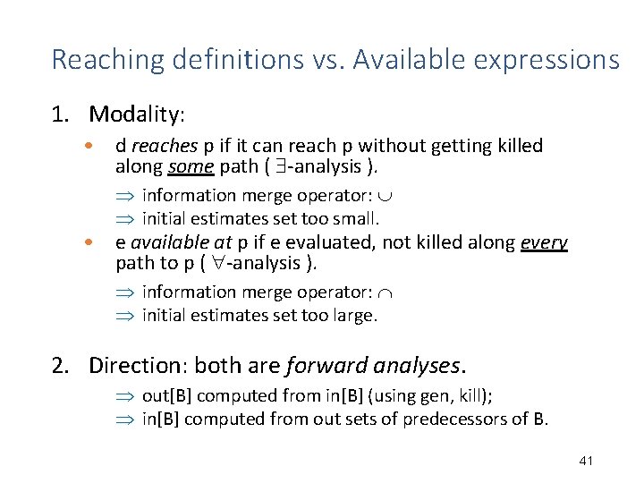
Reaching definitions vs. Available expressions 1. Modality: • d reaches p if it can reach p without getting killed along some path ( -analysis ). information merge operator: initial estimates set too small. • e available at p if e evaluated, not killed along every path to p ( -analysis ). information merge operator: initial estimates set too large. 2. Direction: both are forward analyses. out[B] computed from in[B] (using gen, kill); in[B] computed from out sets of predecessors of B. 41

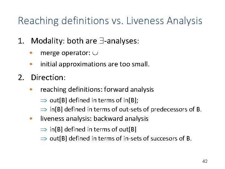
Reaching definitions vs. Liveness Analysis 1. Modality: both are -analyses: • merge operator: • initial approximations are too small. 2. Direction: • reaching definitions: forward analysis out[B] defined in terms of in[B]; in[B] defined in terms of out-sets of predecessors of B. • liveness analysis: backward analysis in[B] defined in terms of out[B] defined in terms of in-sets of succesors of B. 42

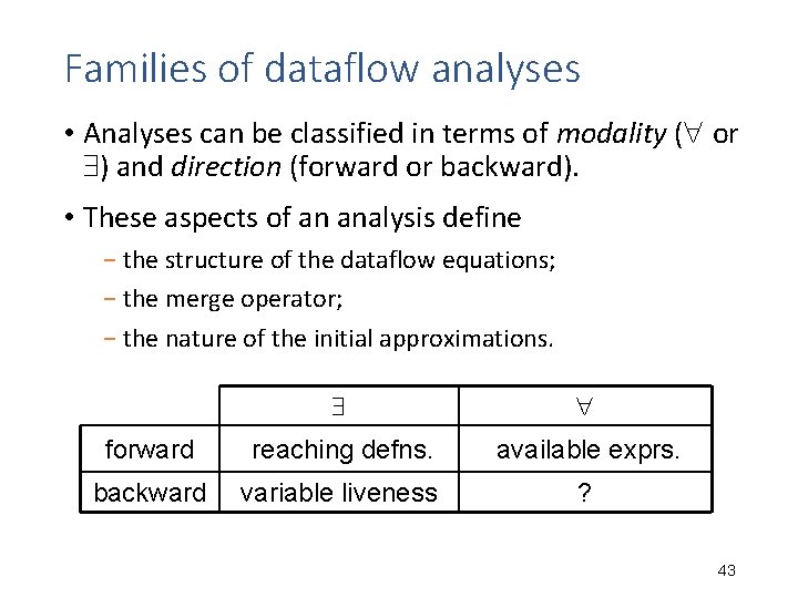
Families of dataflow analyses • Analyses can be classified in terms of modality ( or ) and direction (forward or backward). • These aspects of an analysis define − the structure of the dataflow equations; − the merge operator; − the nature of the initial approximations. forward reaching defns. available exprs. backward variable liveness ? 43

Analysis 4 Constant propagation 44

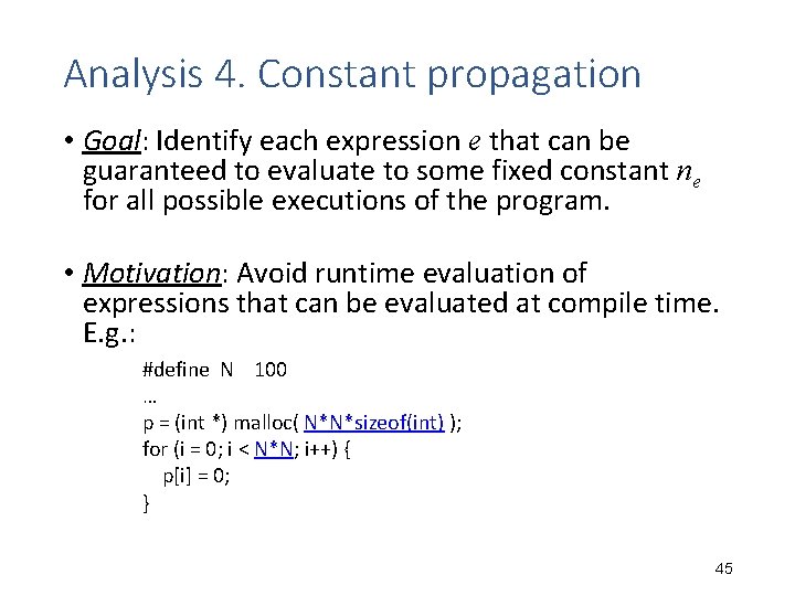
Analysis 4. Constant propagation • Goal: Identify each expression e that can be guaranteed to evaluate to some fixed constant ne for all possible executions of the program. • Motivation: Avoid runtime evaluation of expressions that can be evaluated at compile time. E. g. : #define N 100 … p = (int *) malloc( N*N*sizeof(int) ); for (i = 0; i < N*N; i++) { p[i] = 0; } 45

Constant propagation: Approach • Intuition: Compute an (over-)estimate of the set of values that can be taken on by an expression. − but we really only care about whether or not this set of values is a singleton 46

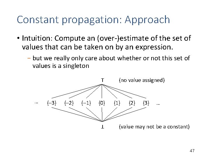
Constant propagation: Approach • Intuition: Compute an (over-)estimate of the set of values that can be taken on by an expression. − but we really only care about whether or not this set of values is a singleton ⊤ … {‒ 3} {‒ 2} {‒ 1} {0} ⊥ (no value assigned) {1} {2} {3} … (value may not be a constant) 47

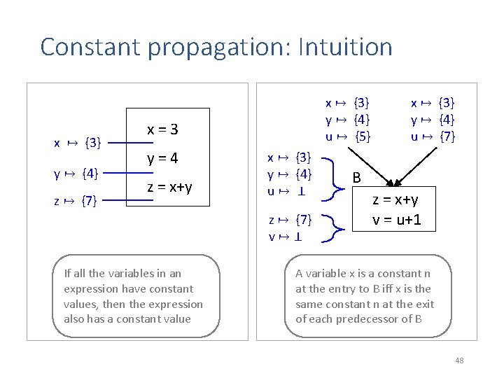
Constant propagation: Intuition x ↦ {3} y ↦ {4} z ↦ {7} x ↦ {3} y ↦ {4} u ↦ {5} x=3 y=4 z = x+y x ↦ {3} y ↦ {4} u↦ ⊥ z ↦ {7} v↦⊥ If all the variables in an expression have constant values, then the expression also has a constant value x ↦ {3} y ↦ {4} u ↦ {7} B z = x+y v = u+1 A variable x is a constant n at the entry to B iff x is the same constant n at the exit of each predecessor of B 48

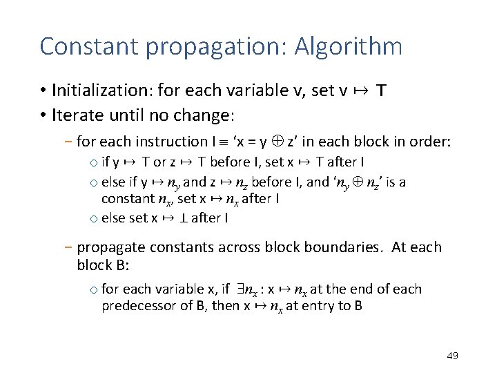
Constant propagation: Algorithm • Initialization: for each variable v, set v ↦ ⊤ • Iterate until no change: − for each instruction I ‘x = y z’ in each block in order: o if y ↦ ⊤ or z ↦ ⊤ before I, set x ↦ ⊤ after I o else if y ↦ ny and z ↦ nz before I, and ‘ny nz’ is a constant nx, set x ↦ nx after I o else set x ↦ ⊥ after I − propagate constants across block boundaries. At each block B: o for each variable x, if nx : x ↦ nx at the end of each predecessor of B, then x ↦ nx at entry to B 49