CSC 550 Introduction to Artificial Intelligence Fall 2008

CSC 550: Introduction to Artificial Intelligence Fall 2008 Connectionist approach to AI § neural networks, neuron model § perceptrons threshold logic, perceptron training, convergence theorem single layer vs. multi-layer § backpropagation stepwise vs. continuous activation function § associative memory Hopfield networks parallel relaxation, relaxation as search 1

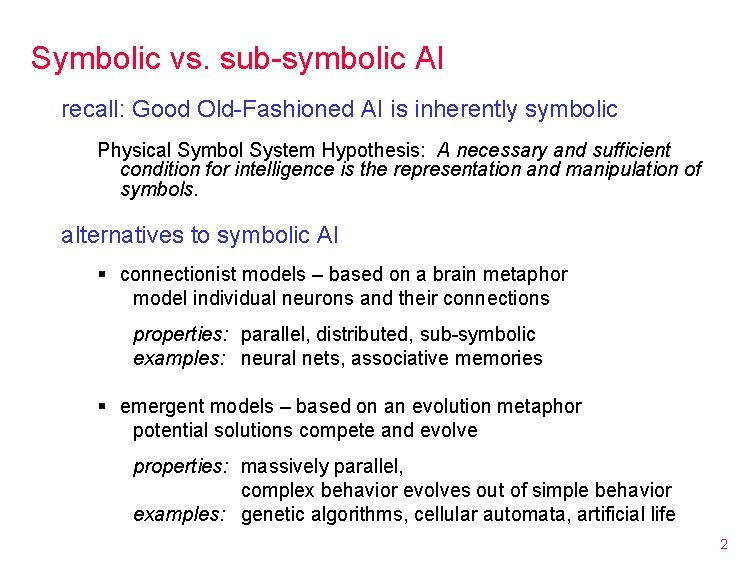
Symbolic vs. sub-symbolic AI recall: Good Old-Fashioned AI is inherently symbolic Physical Symbol System Hypothesis: A necessary and sufficient condition for intelligence is the representation and manipulation of symbols. alternatives to symbolic AI § connectionist models – based on a brain metaphor model individual neurons and their connections properties: parallel, distributed, sub-symbolic examples: neural nets, associative memories § emergent models – based on an evolution metaphor potential solutions compete and evolve properties: massively parallel, complex behavior evolves out of simple behavior examples: genetic algorithms, cellular automata, artificial life 2

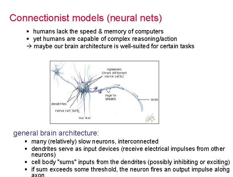
Connectionist models (neural nets) § humans lack the speed & memory of computers § yet humans are capable of complex reasoning/action maybe our brain architecture is well-suited for certain tasks general brain architecture: § many (relatively) slow neurons, interconnected § dendrites serve as input devices (receive electrical impulses from other neurons) § cell body "sums" inputs from the dendrites (possibly inhibiting or exciting) 3 § if sum exceeds some threshold, the neuron fires an output impulse along

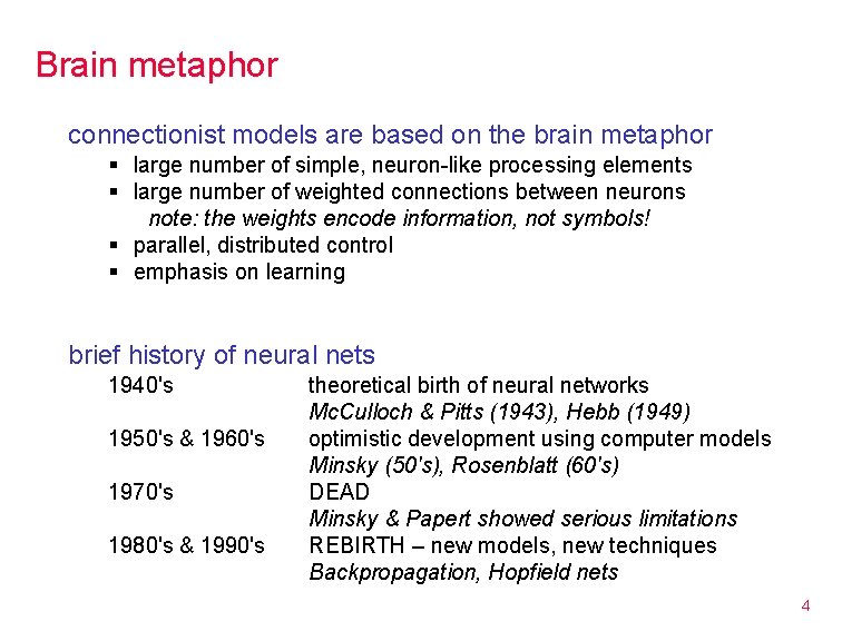
Brain metaphor connectionist models are based on the brain metaphor § large number of simple, neuron-like processing elements § large number of weighted connections between neurons note: the weights encode information, not symbols! § parallel, distributed control § emphasis on learning brief history of neural nets 1940's 1950's & 1960's 1970's 1980's & 1990's theoretical birth of neural networks Mc. Culloch & Pitts (1943), Hebb (1949) optimistic development using computer models Minsky (50's), Rosenblatt (60's) DEAD Minsky & Papert showed serious limitations REBIRTH – new models, new techniques Backpropagation, Hopfield nets 4

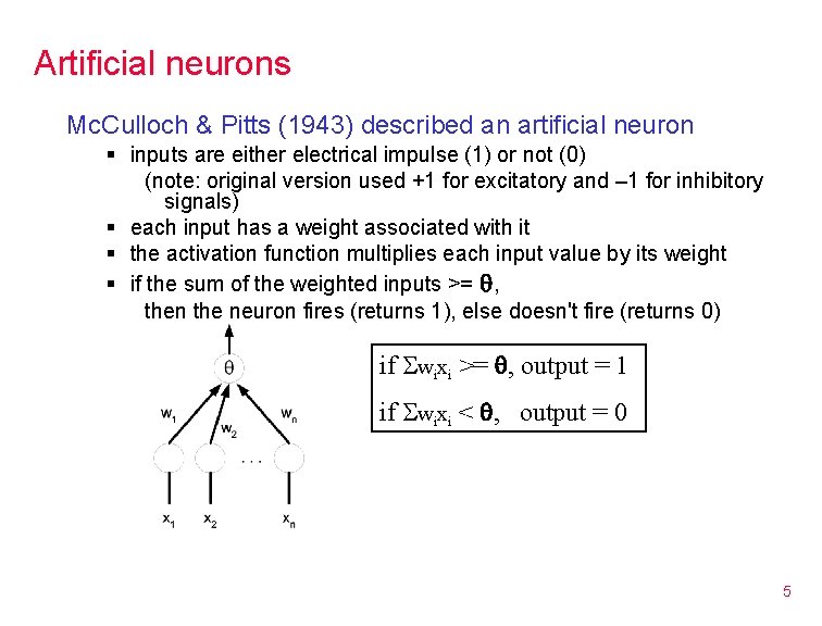
Artificial neurons Mc. Culloch & Pitts (1943) described an artificial neuron § inputs are either electrical impulse (1) or not (0) (note: original version used +1 for excitatory and – 1 for inhibitory signals) § each input has a weight associated with it § the activation function multiplies each input value by its weight § if the sum of the weighted inputs >= , then the neuron fires (returns 1), else doesn't fire (returns 0) if wixi >= , output = 1 if wixi < , output = 0 5

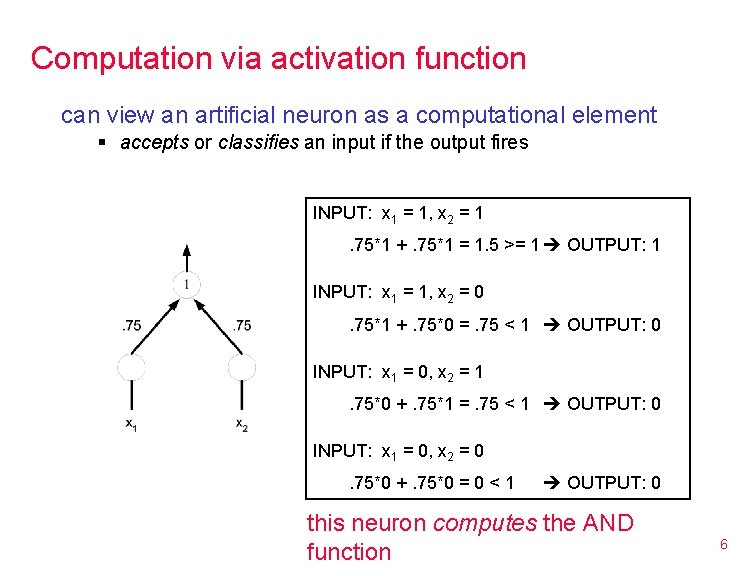
Computation via activation function can view an artificial neuron as a computational element § accepts or classifies an input if the output fires INPUT: x 1 = 1, x 2 = 1. 75*1 +. 75*1 = 1. 5 >= 1 OUTPUT: 1 INPUT: x 1 = 1, x 2 = 0. 75*1 +. 75*0 =. 75 < 1 OUTPUT: 0 INPUT: x 1 = 0, x 2 = 1. 75*0 +. 75*1 =. 75 < 1 OUTPUT: 0 INPUT: x 1 = 0, x 2 = 0. 75*0 +. 75*0 = 0 < 1 OUTPUT: 0 this neuron computes the AND function 6

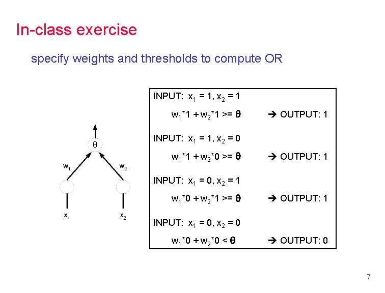
In-class exercise specify weights and thresholds to compute OR INPUT: x 1 = 1, x 2 = 1 w 1*1 + w 2*1 >= OUTPUT: 1 INPUT: x 1 = 1, x 2 = 0 w 1*1 + w 2*0 >= OUTPUT: 1 INPUT: x 1 = 0, x 2 = 1 w 1*0 + w 2*1 >= OUTPUT: 1 INPUT: x 1 = 0, x 2 = 0 w 1*0 + w 2*0 < OUTPUT: 0 7

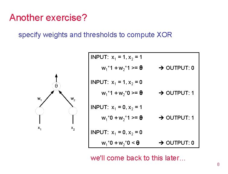
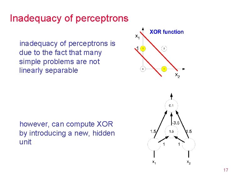
Another exercise? specify weights and thresholds to compute XOR INPUT: x 1 = 1, x 2 = 1 w 1*1 + w 2*1 >= OUTPUT: 0 INPUT: x 1 = 1, x 2 = 0 w 1*1 + w 2*0 >= OUTPUT: 1 INPUT: x 1 = 0, x 2 = 1 w 1*0 + w 2*1 >= OUTPUT: 1 INPUT: x 1 = 0, x 2 = 0 w 1*0 + w 2*0 < OUTPUT: 0 we'll come back to this later… 8

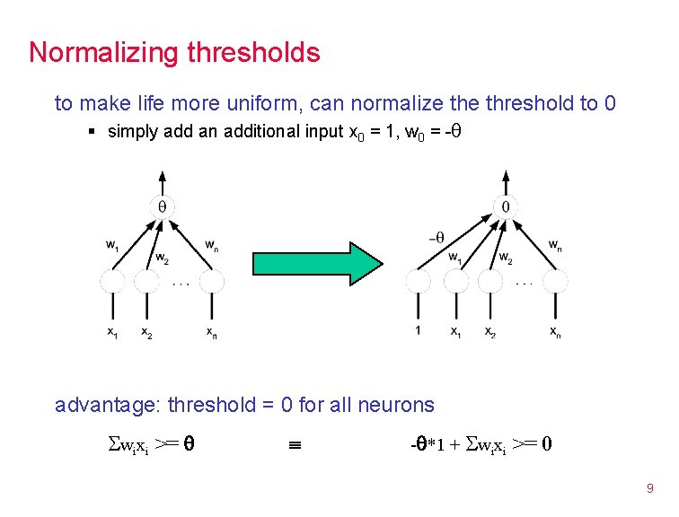
Normalizing thresholds to make life more uniform, can normalize threshold to 0 § simply add an additional input x 0 = 1, w 0 = - advantage: threshold = 0 for all neurons wixi >= - *1 + wixi >= 0 9

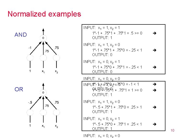
Normalized examples AND OR INPUT: x 1 = 1, x 2 = 1 1*-1 +. 75*1 =. 5 >= 0 OUTPUT: 1 INPUT: x 1 = 1, x 2 = 0 1*-1 +. 75*0 = -. 25 < 1 OUTPUT: 0 INPUT: x 1 = 0, x 2 = 1 1*-1 +. 75*0 +. 75*1 = -. 25 < 1 OUTPUT: 0 INPUT: x 1 = 0, x 2 = 0 1*-1 x 1+. 75*0 = -1 < 1 INPUT: = 1, x 2+=. 75*0 1 OUTPUT: 0 +. 75*1 = 1 >= 0 1*-. 5 +. 75*1 OUTPUT: 1 INPUT: x 1 = 1, x 2 = 0 1*-. 5 +. 75*1 +. 75*0 =. 25 > 1 OUTPUT: 1 INPUT: x 1 = 0, x 2 = 1 1*-. 5 +. 75*0 +. 75*1 =. 25 < 1 OUTPUT: 1 INPUT: x 1 = 0, x 2 = 0 10

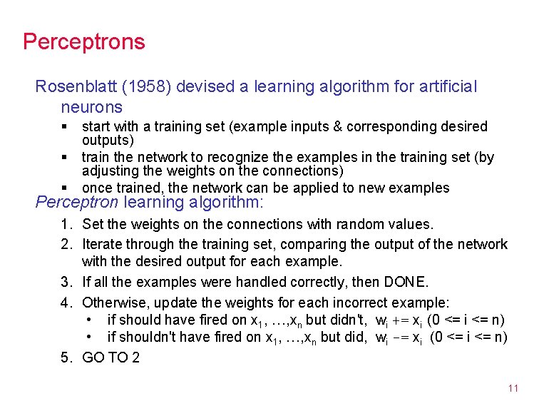
Perceptrons Rosenblatt (1958) devised a learning algorithm for artificial neurons § § § start with a training set (example inputs & corresponding desired outputs) train the network to recognize the examples in the training set (by adjusting the weights on the connections) once trained, the network can be applied to new examples Perceptron learning algorithm: 1. Set the weights on the connections with random values. 2. Iterate through the training set, comparing the output of the network with the desired output for each example. 3. If all the examples were handled correctly, then DONE. 4. Otherwise, update the weights for each incorrect example: • if should have fired on x 1, …, xn but didn't, wi += xi (0 <= i <= n) • if shouldn't have fired on x 1, …, xn but did, wi -= xi (0 <= i <= n) 5. GO TO 2 11

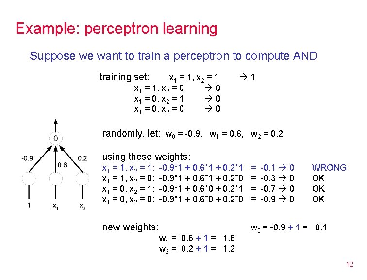
Example: perceptron learning Suppose we want to train a perceptron to compute AND training set: x 1 = 1, x 2 = 1 x 1 = 1, x 2 = 0 0 x 1 = 0, x 2 = 1 0 x 1 = 0, x 2 = 0 0 1 randomly, let: w 0 = -0. 9, w 1 = 0. 6, w 2 = 0. 2 using these weights: x 1 = 1, x 2 = 1: x 1 = 1, x 2 = 0: x 1 = 0, x 2 = 1: x 1 = 0, x 2 = 0: -0. 9*1 + 0. 6*1 + 0. 2*1 -0. 9*1 + 0. 6*1 + 0. 2*0 -0. 9*1 + 0. 6*0 + 0. 2*1 -0. 9*1 + 0. 6*0 + 0. 2*0 new weights: w 1 = 0. 6 + 1 = 1. 6 w 2 = 0. 2 + 1 = 1. 2 = = -0. 1 0 -0. 3 0 -0. 7 0 -0. 9 0 WRONG OK OK OK w 0 = -0. 9 + 1 = 0. 1 12

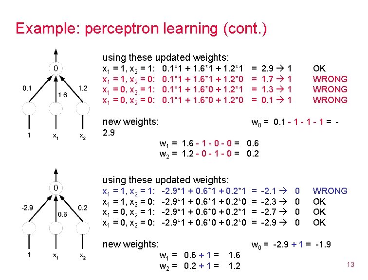
Example: perceptron learning (cont. ) using these updated weights: x 1 = 1, x 2 = 1: x 1 = 1, x 2 = 0: x 1 = 0, x 2 = 1: x 1 = 0, x 2 = 0: 0. 1*1 + 1. 6*1 + 1. 2*1 0. 1*1 + 1. 6*1 + 1. 2*0 0. 1*1 + 1. 6*0 + 1. 2*1 0. 1*1 + 1. 6*0 + 1. 2*0 new weights: = = 2. 9 1 1. 7 1 1. 3 1 0. 1 1 OK WRONG w 0 = 0. 1 - 1 - 1 = - 2. 9 w 1 = 1. 6 - 1 - 0 = 0. 6 w 2 = 1. 2 - 0 - 1 - 0 = 0. 2 using these updated weights: x 1 = 1, x 2 = 1: x 1 = 1, x 2 = 0: x 1 = 0, x 2 = 1: x 1 = 0, x 2 = 0: -2. 9*1 + 0. 6*1 + 0. 2*1 -2. 9*1 + 0. 6*1 + 0. 2*0 -2. 9*1 + 0. 6*0 + 0. 2*1 -2. 9*1 + 0. 6*0 + 0. 2*0 new weights: w 1 = 0. 6 + 1 = w 2 = 0. 2 + 1 = 1. 6 1. 2 = = -2. 1 -2. 3 -2. 7 -2. 9 0 0 WRONG OK OK OK w 0 = -2. 9 + 1 = -1. 9 13

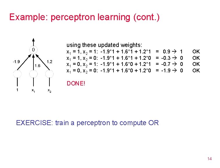
Example: perceptron learning (cont. ) using these updated weights: x 1 = 1, x 2 = 1: x 1 = 1, x 2 = 0: x 1 = 0, x 2 = 1: x 1 = 0, x 2 = 0: -1. 9*1 + 1. 6*1 + 1. 2*1 -1. 9*1 + 1. 6*1 + 1. 2*0 -1. 9*1 + 1. 6*0 + 1. 2*1 -1. 9*1 + 1. 6*0 + 1. 2*0 = = 0. 9 -0. 3 -0. 7 -1. 9 1 0 0 0 OK OK DONE! EXERCISE: train a perceptron to compute OR 14

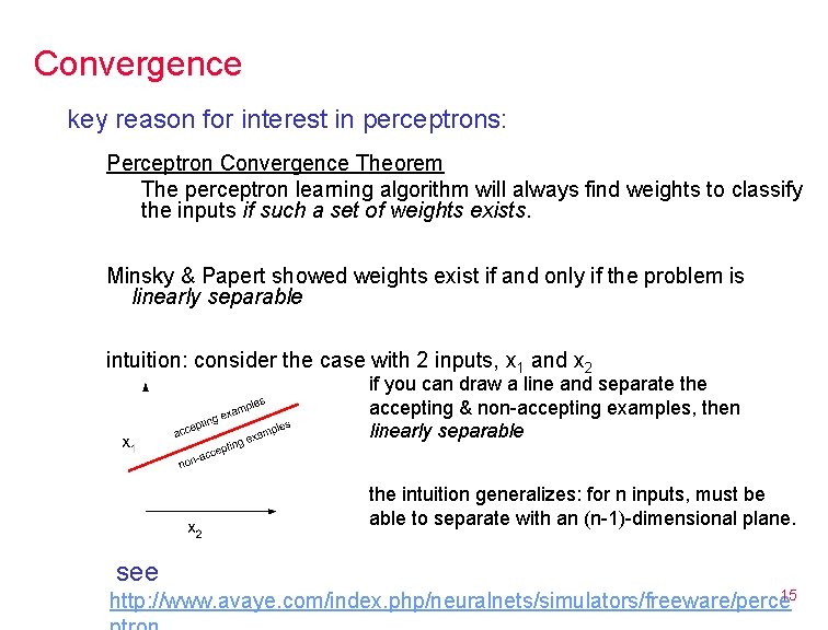
Convergence key reason for interest in perceptrons: Perceptron Convergence Theorem The perceptron learning algorithm will always find weights to classify the inputs if such a set of weights exists. Minsky & Papert showed weights exist if and only if the problem is linearly separable intuition: consider the case with 2 inputs, x 1 and x 2 if you can draw a line and separate the accepting & non-accepting examples, then linearly separable the intuition generalizes: for n inputs, must be able to separate with an (n-1)-dimensional plane. see http: //www. avaye. com/index. php/neuralnets/simulators/freeware/perce 15

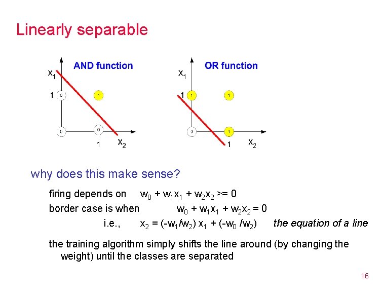
Linearly separable why does this make sense? firing depends on w 0 + w 1 x 1 + w 2 x 2 >= 0 border case is when w 0 + w 1 x 1 + w 2 x 2 = 0 i. e. , x 2 = (-w 1/w 2) x 1 + (-w 0 /w 2) the equation of a line the training algorithm simply shifts the line around (by changing the weight) until the classes are separated 16

Inadequacy of perceptrons is due to the fact that many simple problems are not linearly separable however, can compute XOR by introducing a new, hidden unit 17

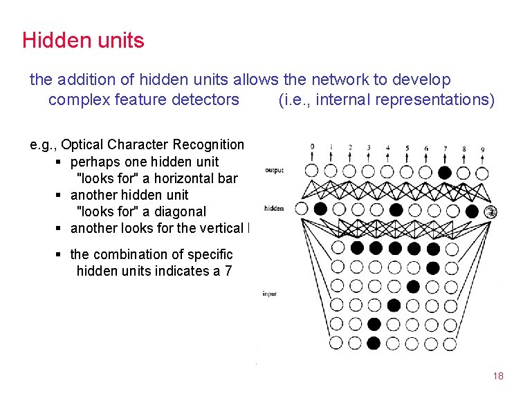
Hidden units the addition of hidden units allows the network to develop complex feature detectors (i. e. , internal representations) e. g. , Optical Character Recognition (OCR) § perhaps one hidden unit "looks for" a horizontal bar § another hidden unit "looks for" a diagonal § another looks for the vertical base § the combination of specific hidden units indicates a 7 18

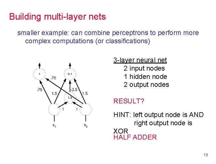
Building multi-layer nets smaller example: can combine perceptrons to perform more complex computations (or classifications) 3 -layer neural net 2 input nodes 1 hidden node 2 output nodes RESULT? HINT: left output node is AND right output node is XOR HALF ADDER 19

Hidden units & learning every classification problem has a perceptron solution if enough hidden layers are used § i. e. , multi-layer networks can compute anything (recall: can simulate AND, OR, NOT gates) expressiveness is not the problem – learning is! § it is not known how to systematically find solutions § the Perceptron Learning Algorithm can't adjust weights between levels Minsky & Papert's results about the "inadequacy" of perceptrons pretty much killed neural net research in the 1970's rebirth in the 1980's due to several developments § faster, more parallel computers § new learning algorithms e. g. , backpropagation § new architectures e. g. , Hopfield nets 20

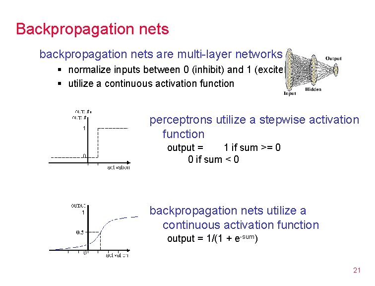
Backpropagation nets backpropagation nets are multi-layer networks § normalize inputs between 0 (inhibit) and 1 (excite) § utilize a continuous activation function perceptrons utilize a stepwise activation function output = 1 if sum >= 0 0 if sum < 0 backpropagation nets utilize a continuous activation function output = 1/(1 + e-sum) 21

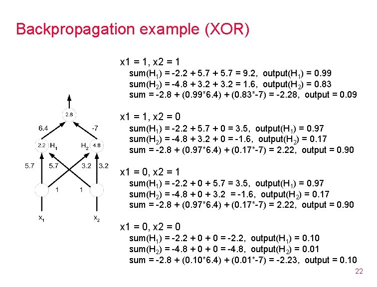
Backpropagation example (XOR) x 1 = 1, x 2 = 1 sum(H 1) = -2. 2 + 5. 7 = 9. 2, output(H 1) = 0. 99 sum(H 2) = -4. 8 + 3. 2 = 1. 6, output(H 2) = 0. 83 sum = -2. 8 + (0. 99*6. 4) + (0. 83*-7) = -2. 28, output = 0. 09 x 1 = 1, x 2 = 0 sum(H 1) = -2. 2 + 5. 7 + 0 = 3. 5, output(H 1) = 0. 97 sum(H 2) = -4. 8 + 3. 2 + 0 = -1. 6, output(H 2) = 0. 17 sum = -2. 8 + (0. 97*6. 4) + (0. 17*-7) = 2. 22, output = 0. 90 x 1 = 0, x 2 = 1 sum(H 1) = -2. 2 + 0 + 5. 7 = 3. 5, output(H 1) = 0. 97 sum(H 2) = -4. 8 + 0 + 3. 2 = -1. 6, output(H 2) = 0. 17 sum = -2. 8 + (0. 97*6. 4) + (0. 17*-7) = 2. 22, output = 0. 90 x 1 = 0, x 2 = 0 sum(H 1) = -2. 2 + 0 = -2. 2, output(H 1) = 0. 10 sum(H 2) = -4. 8 + 0 = -4. 8, output(H 2) = 0. 01 sum = -2. 8 + (0. 10*6. 4) + (0. 01*-7) = -2. 23, output = 0. 10 22

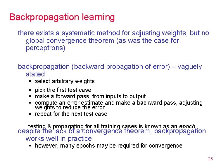
Backpropagation learning there exists a systematic method for adjusting weights, but no global convergence theorem (as was the case for perceptrons) backpropagation (backward propagation of error) – vaguely stated § § select arbitrary weights pick the first test case make a forward pass, from inputs to output compute an error estimate and make a backward pass, adjusting weights to reduce the error § repeat for the next test case testing & propagating for all training cases is known as an epoch despite the lack of a convergence theorem, backpropagation works well in practice § however, many epochs may be required for convergence 23

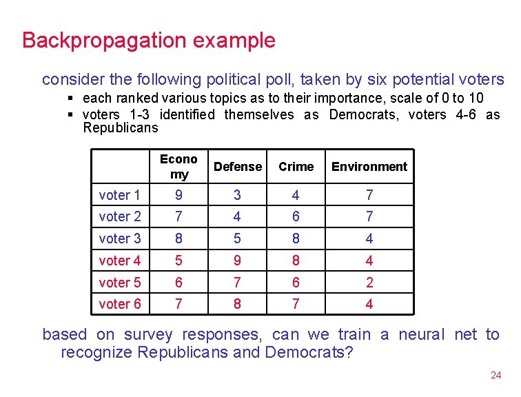
Backpropagation example consider the following political poll, taken by six potential voters § each ranked various topics as to their importance, scale of 0 to 10 § voters 1 -3 identified themselves as Democrats, voters 4 -6 as Republicans Econo my Defense Crime Environment voter 1 9 3 4 7 voter 2 7 4 6 7 voter 3 8 5 8 4 voter 4 5 9 8 4 voter 5 6 7 6 2 voter 6 7 8 7 4 based on survey responses, can we train a neural net to recognize Republicans and Democrats? 24

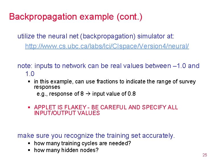
Backpropagation example (cont. ) utilize the neural net (backpropagation) simulator at: http: //www. cs. ubc. ca/labs/lci/CIspace/Version 4/neural/ note: inputs to network can be real values between – 1. 0 and 1. 0 § in this example, can use fractions to indicate the range of survey responses e. g. , response of 8 input value of 0. 8 § APPLET IS FLAKEY - BE CAREFUL AND SPECIFY ALL INPUT/OUTPUT VALUES make sure you recognize the training set accurately. § how many training cycles are needed? § how many hidden nodes? 25

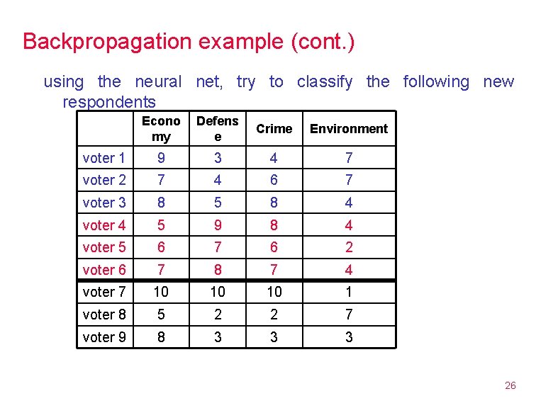
Backpropagation example (cont. ) using the neural net, try to classify the following new respondents Econo my Defens e Crime Environment voter 1 9 3 4 7 voter 2 7 4 6 7 voter 3 8 5 8 4 voter 4 5 9 8 4 voter 5 6 7 6 2 voter 6 7 8 7 4 voter 7 10 10 10 1 voter 8 5 2 2 7 voter 9 8 3 3 3 26

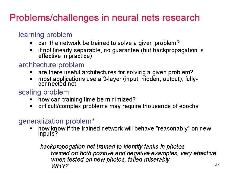
Problems/challenges in neural nets research learning problem § § can the network be trained to solve a given problem? if not linearly separable, no guarantee (but backpropagation is effective in practice) architecture problem § § are there useful architectures for solving a given problem? most applications use a 3 -layer (input, hidden, output), fullyconnected net scaling problem § § how can training time be minimized? difficult/complex problems may require thousands of epochs generalization problem* § how know if the trained network will behave "reasonably" on new inputs? backpropogation net trained to identify tanks in photos trained on both positive and negative examples, very effective when tested on new photos, failed miserably 27 WHY?

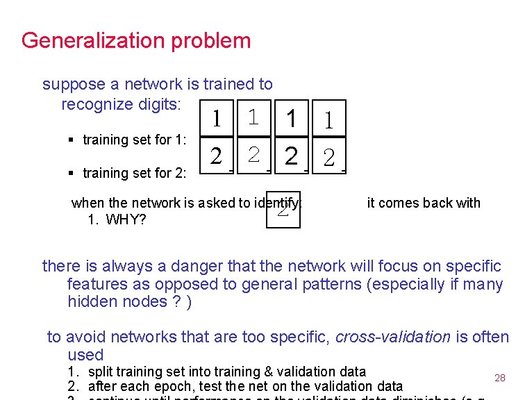
Generalization problem suppose a network is trained to recognize digits: § training set for 1: § training set for 2: 1 1 2 2 when the network is asked to identify: 1. WHY? 2 it comes back with there is always a danger that the network will focus on specific features as opposed to general patterns (especially if many hidden nodes ? ) to avoid networks that are too specific, cross-validation is often used 1. split training set into training & validation data 2. after each epoch, test the net on the validation data 28

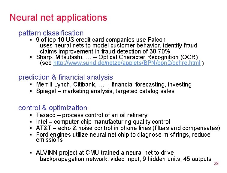
Neural net applications pattern classification § 9 of top 10 US credit card companies use Falcon uses neural nets to model customer behavior, identify fraud claims improvement in fraud detection of 30 -70% § Sharp, Mitsubishi, … -- Optical Character Recognition (OCR) (see http: //www. sund. de/netze/applets/BPN/bpn 2/ochre. html ) prediction & financial analysis § Merrill Lynch, Citibank, … -- financial forecasting, investing § Spiegel – marketing analysis, targeted catalog sales control & optimization § § Texaco – process control of an oil refinery Intel – computer chip manufacturing quality control AT&T – echo & noise control in phone lines (filters and compensates) Ford engines utilize neural net chip to diagnose misfirings, reduce emissions § ALVINN project at CMU trained a neural net to drive backpropagation network: video input, 9 hidden units, 45 outputs 29

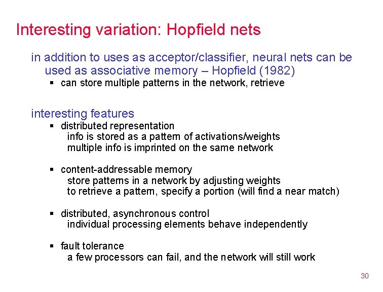
Interesting variation: Hopfield nets in addition to uses as acceptor/classifier, neural nets can be used as associative memory – Hopfield (1982) § can store multiple patterns in the network, retrieve interesting features § distributed representation info is stored as a pattern of activations/weights multiple info is imprinted on the same network § content-addressable memory store patterns in a network by adjusting weights to retrieve a pattern, specify a portion (will find a near match) § distributed, asynchronous control individual processing elements behave independently § fault tolerance a few processors can fail, and the network will still work 30

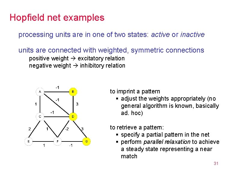
Hopfield net examples processing units are in one of two states: active or inactive units are connected with weighted, symmetric connections positive weight excitatory relation negative weight inhibitory relation to imprint a pattern § adjust the weights appropriately (no general algorithm is known, basically ad. hoc) to retrieve a pattern: § specify a partial pattern in the net § perform parallel relaxation to achieve a steady state representing a near match 31

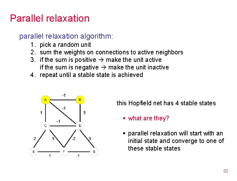
Parallel relaxation parallel relaxation algorithm: 1. pick a random unit 2. sum the weights on connections to active neighbors 3. if the sum is positive make the unit active if the sum is negative make the unit inactive 4. repeat until a stable state is achieved this Hopfield net has 4 stable states § what are they? § parallel relaxation will start with an initial state and converge to one of these stable states 32

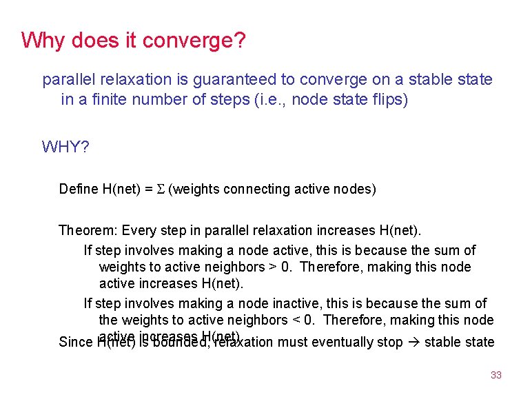
Why does it converge? parallel relaxation is guaranteed to converge on a stable state in a finite number of steps (i. e. , node state flips) WHY? Define H(net) = (weights connecting active nodes) Theorem: Every step in parallel relaxation increases H(net). If step involves making a node active, this is because the sum of weights to active neighbors > 0. Therefore, making this node active increases H(net). If step involves making a node inactive, this is because the sum of the weights to active neighbors < 0. Therefore, making this node active increases H(net). Since H(net) is bounded, relaxation must eventually stop stable state 33

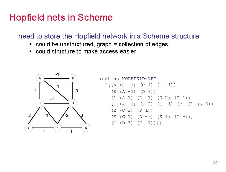
Hopfield nets in Scheme need to store the Hopfield network in a Scheme structure § could be unstructured, graph = collection of edges § could structure to make access easier (define HOPFIELD-NET '((A (B -1) (C 1) (D (B (A -1) (D 3)) (C (A 1) (D -1) (E (D (A -1) (B 3) (C (E (C 2) (F 1)) (F (C 1) (D -2) (E (G (D 3) (F -1)))) -1)) 2) (F 1)) -1) (F -2) (G 3)) 1) (G -1)) 34

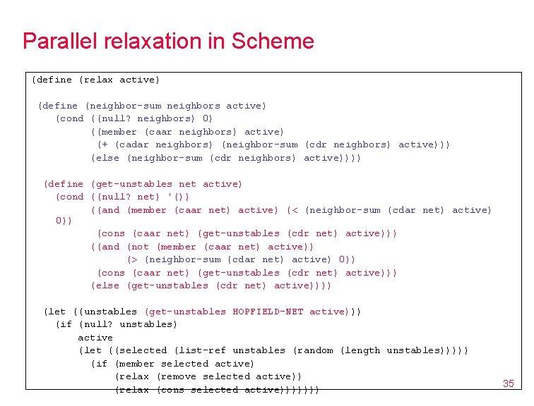
Parallel relaxation in Scheme (define (relax active) (define (neighbor-sum neighbors active) (cond ((null? neighbors) 0) ((member (caar neighbors) active) (+ (cadar neighbors) (neighbor-sum (cdr neighbors) active))) (else (neighbor-sum (cdr neighbors) active)))) (define (get-unstables net active) (cond ((null? net) '()) ((and (member (caar net) active) (< (neighbor-sum (cdar net) active) 0)) (cons (caar net) (get-unstables (cdr net) active))) ((and (not (member (caar net) active)) (> (neighbor-sum (cdar net) active) 0)) (cons (caar net) (get-unstables (cdr net) active))) (else (get-unstables (cdr net) active)))) (let ((unstables (get-unstables HOPFIELD-NET active))) (if (null? unstables) active (let ((selected (list-ref unstables (random (length unstables))))) (if (member selected active) (relax (remove selected active)) (relax (cons selected active))))))) 35

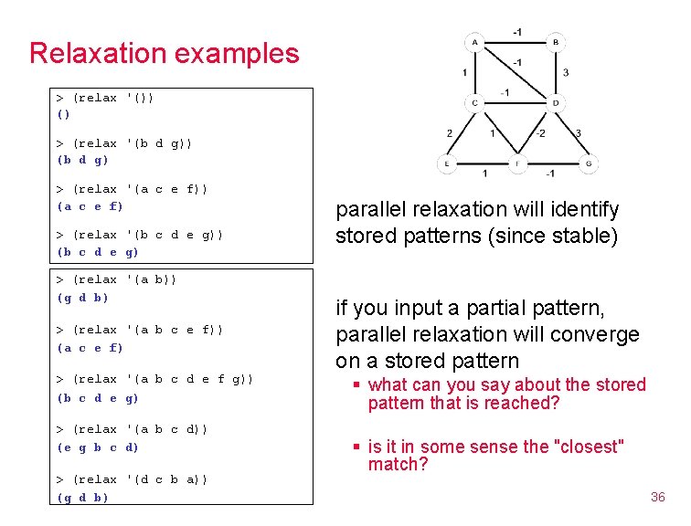
Relaxation examples > (relax '()) () > (relax '(b d g)) (b d g) > (relax '(a c e f)) (a c e f) > (relax '(b c d e g)) (b c d e g) > (relax '(a b)) (g d b) > (relax '(a b c e f)) (a c e f) > (relax '(a b c d e f g)) (b c d e g) > (relax '(a b c d)) (e g b c d) > (relax '(d c b a)) (g d b) parallel relaxation will identify stored patterns (since stable) if you input a partial pattern, parallel relaxation will converge on a stored pattern § what can you say about the stored pattern that is reached? § is it in some sense the "closest" match? 36

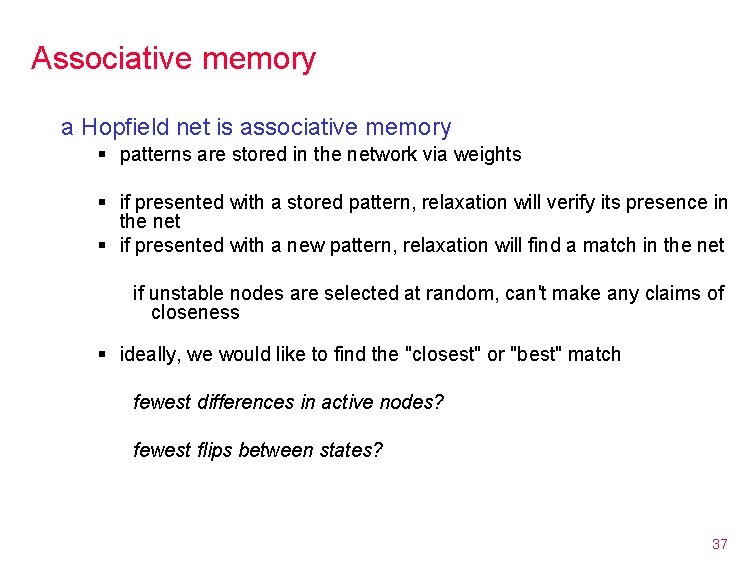
Associative memory a Hopfield net is associative memory § patterns are stored in the network via weights § if presented with a stored pattern, relaxation will verify its presence in the net § if presented with a new pattern, relaxation will find a match in the net if unstable nodes are selected at random, can't make any claims of closeness § ideally, we would like to find the "closest" or "best" match fewest differences in active nodes? fewest flips between states? 37

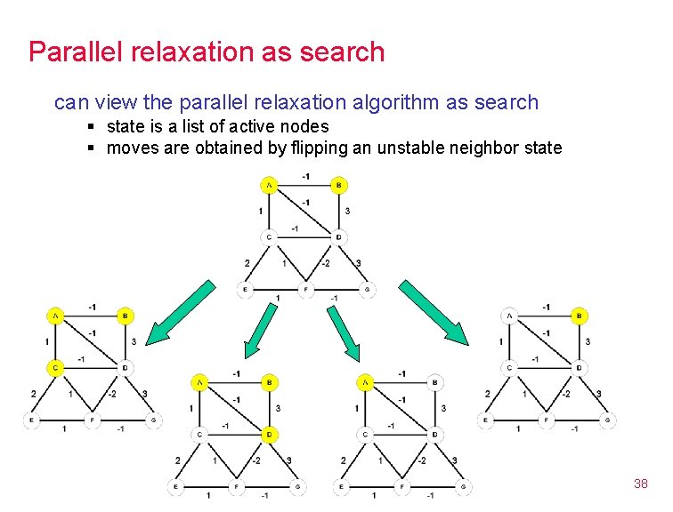
Parallel relaxation as search can view the parallel relaxation algorithm as search § state is a list of active nodes § moves are obtained by flipping an unstable neighbor state 38

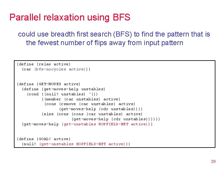
Parallel relaxation using BFS could use breadth first search (BFS) to find the pattern that is the fewest number of flips away from input pattern (define (relax active) (car (bfs-nocycles active))) (define (GET-MOVES active) (define (get-moves-help unstables) (cond ((null? unstables) '()) ((member (car unstables) active) (cons (remove (car unstables) active) (get-moves-help (cdr unstables)))) (else (cons (car unstables) active) (get-moves-help (cdr unstables)))))) (get-moves-help (get-unstables HOPFIELD-NET active))) (define (GOAL? active) (null? (get-unstables HOPFIELD-NET active))) 39

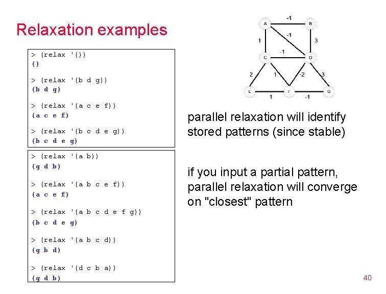
Relaxation examples > (relax '()) () > (relax '(b d g)) (b d g) > (relax '(a c e f)) (a c e f) > (relax '(b c d e g)) (b c d e g) > (relax '(a b)) (g d b) > (relax '(a b c e f)) (a c e f) parallel relaxation will identify stored patterns (since stable) if you input a partial pattern, parallel relaxation will converge on "closest" pattern > (relax '(a b c d e f g)) (b c d e g) > (relax '(a b c d)) (g b d) > (relax '(d c b a)) (g d b) 40

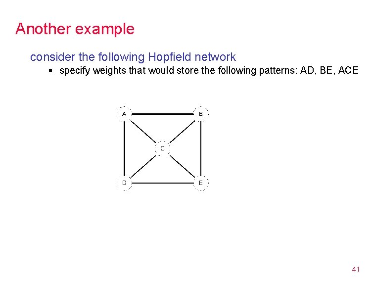
Another example consider the following Hopfield network § specify weights that would store the following patterns: AD, BE, ACE 41

Additional readings Neural Network from Wikipedia NN applications from Stanford Applications of adaptive systems from Peltarion MSN Search's Ranking Algorithm uses a Neural Net by Richard Drawhorn Recognition of face profiles from the MUGSHOT database using a hybrid connectionist/hmm approach by Wallhoff, Muller, and Rigoll 42