CSC 480 ARTIFICIAL INTELLIGENCE BAMSHAD MOBASHER CONSTRAINT SATISFACTION

CSC 480 ARTIFICIAL INTELLIGENCE BAMSHAD MOBASHER CONSTRAINT SATISFACTION PROBLEMS

WHAT IS SEARCH FOR? • Assumptions about the world: a single agent, deterministic actions, fully observed state, discrete state space • Planning: sequences of actions • • • The path to the goal is the important thing Paths have various costs, depths Heuristics give problem-specific guidance • Identification: assignments to variables • • The goal itself is important, not the path CSPs: specialized form of search problems for identification problems

QUEENS PUZZLE • Place eight queens on a chessboard so that no two attack each other Q Q Q Q

SEARCH FORMULATION OF THE QUEENS PUZZLE • Successors: all valid ways of placing additional queen on the board; goal: eight queens placed Q Q Q Q Q Q Q Q Q

• • CONSTRAINT SATISFACTION PROBLEMS Standard search problems: • • • Constraint satisfaction problems (CSPs): • • State is a “black box”: arbitrary data structure Goal test can be any function over states Successor function can also be anything A special subset of search problems State is defined by variables Xi with values from a domain D (sometimes D depends on i) Goal test is a set of constraints specifying allowable combinations of values for subsets of variables Allows useful general-purpose algorithms with more power than standard search algorithms

CONSTRAINT SATISFACTION PROBLEMS • An assignment is complete when every variable is accounted for • A solution to a CSP is a complete assignment that satisfies all constraints • Some CSPs require a solution that maximizes an objective function • Examples of Applications: • Scheduling the time of observations on the Hubble Space Telescope • Airline schedules • Cryptography • Course planning

CSP EXAMPLES

EXAMPLE: MAP COLORING • Variables: • Domains: • Constraints: adjacent regions must have different colors Implicit: Explicit: • Solutions are assignments satisfying all constraints, e. g. :

EXAMPLE: N-QUEENS • Formulation 1: • • • Variables: Domains: Constraints (each square)

EXAMPLE: N-QUEENS 1 2 • Formulation 2: • Variables: • Domains: • Constraints: Implicit: Explicit: (location of queen on row k 3 4

EXAMPLE: SUDOKU Variables: Each (open) square Domains: {1, 2, …, 9} Constraints: 9 -way alldiff for each column 9 -way alldiff for each row 9 -way alldiff for each region (or can have a bunch of pairwise inequality constraints)

EXAMPLE: SUDOKU

CONSTRAINT GRAPHS • Binary CSP: each constraint relates (at most) two variables • Binary constraint graph: nodes are variables, arcs show constraints • General-purpose CSP algorithms use the graph structure to speed up search. E. g. , Tasmania is an independent subproblem!

EXAMPLE: CRYPTARITHMETIC • Variables: • Domains: • Constraints:

VARIETIES OF CSPS • Discrete variables • Finite domains; size d O(dn) complete assignments. • E. g. Boolean CSPs: Boolean satisfiability (NP-complete). • Infinite domains (integers, strings, etc. ) • • • E. g. job scheduling, variables are start/end days for each job Need a constraint language e. g Start. Job 1 +5 ≤ Start. Job 3. Infinitely many solutions Linear constraints: solvable Nonlinear: no general algorithm • Continuous variables • e. g. building an airline schedule or class schedule. • Linear constraints solvable in polynomial time by LP methods.

VARIETIES OF CONSTRAINTS • Unary constraints involve a single variable. • e. g. SA green • Binary constraints involve pairs of variables. • e. g. SA WA • Higher-order constraints involve 3 or more variables. • Professors A, B, and C cannot be on a committee together • Can always be represented by multiple binary constraints • Preference (soft constraints) • e. g. red is better than green • often can be represented by a cost for each variable assignment • combination of optimization with CSPs

STANDARD SEARCH FORMULATION • CSPs can be expressed as a standard search problem • States defined by the values assigned so far (partial assignments) • Initial state: the empty assignment, {} • Successor function: assign a value to an • unassigned variable Goal test: the current assignment is complete and satisfies all constraints • We’ll start with the straightforward, naïve approach, then improve it

CSP AS A STANDARD SEARCH PROBLEM • Solution is found at depth n (if there are n variables). • Consider using BFS • Branching factor b at the top level is n x d • At next level is (n-1) x d • …. • End up with n!dn leaves even though there are only dn complete assignments!

BACKTRACKING SEARCH • The basic uninformed algorithm for solving CSPs • Idea 1: One variable at a time • Variable assignments are commutative, so fix ordering • I. e. , [WA = red then NT = green] same as [NT = green then WA = red] • Only need to consider assignments to a single variable at each step • Idea 2: Check constraints as you go • I. e. consider only values which do not conflict previous assignments • Might have to do some computation to check the constraints • “Incremental goal test” • Depth-first search with these two improvements is called backtracking search (not the best name) • Can solve n-queens for n 25

BACKTRACKING EXAMPLE

BACKTRACKING SEARCH • Backtracking = DFS + variable-ordering + fail-on-violation

IMPROVING BACKTRACKING • General-purpose ideas give huge gains in speed • Ordering: • Which variable should be assigned next? • In what order should its values be tried? • Filtering: Can we detect inevitable failure early? • Structure: Can we exploit the problem structure?

FILTERING

FILTERING: FORWARD CHECKING • Filtering: Keep track of domains for unassigned variables and cross off bad options • Forward checking: Cross off values that violate a constraint when added to the existing assignment

FORWARD CHECKING • Assign {WA=red} • Effects on other variables connected by constraints to WA • • NT can no longer be red SA can no longer be red

FORWARD CHECKING • Assign {Q=green} • Effects on other variables connected by constraints with Q • • • NT can no longer be green NSW can no longer be green SA can no longer be green

FORWARD CHECKING • If V is assigned blue • Effects on other variables connected by constraints with V • • • NSW can no longer be blue SA is empty FC has detected that partial assignment is inconsistent with the constraints and backtracking can occur.

EXAMPLE: 4 -QUEENS PROBLEM 1 2 3 4 X 1 {1, 2, 3, 4} X 2 {1, 2, 3, 4} X 3 {1, 2, 3, 4} X 4 {1, 2, 3, 4} 1 2 3 4

EXAMPLE: 4 -QUEENS PROBLEM 1 2 3 4 X 1 {1, 2, 3, 4} X 2 {1, 2, 3, 4} X 3 {1, 2, 3, 4} X 4 {1, 2, 3, 4} 1 2 3 4

EXAMPLE: 4 -QUEENS PROBLEM 1 2 3 4 X 1 {1, 2, 3, 4} X 2 { , , 3, 4} X 3 { , 2, , 4} X 4 { , 2, 3, } 1 2 3 4

EXAMPLE: 4 -QUEENS PROBLEM 1 2 3 4 X 1 {1, 2, 3, 4} X 2 { , , 3, 4} X 3 { , 2, , 4} X 4 { , 2, 3, } 1 2 3 4

EXAMPLE: 4 -QUEENS PROBLEM 1 2 3 4 X 1 {1, 2, 3, 4} X 2 { , , 3, 4} X 3 { , , , } X 4 { , , 3, } 1 2 3 4

EXAMPLE: 4 -QUEENS PROBLEM 1 2 3 4 X 1 {1, 2, 3, 4} X 2 { , , , 4} X 3 { , 2, , 4} X 4 { , 2, 3, } 1 2 3 4

EXAMPLE: 4 -QUEENS PROBLEM 1 2 3 4 X 1 {1, 2, 3, 4} X 2 { , , , 4} X 3 { , 2, , 4} X 4 { , 2, 3, } 1 2 3 4

EXAMPLE: 4 -QUEENS PROBLEM 1 2 3 4 X 1 {1, 2, 3, 4} X 2 { , , , 4} X 3 { , 2, , } X 4 { , , 3, } 1 2 3 4

EXAMPLE: 4 -QUEENS PROBLEM 1 2 3 4 X 1 {1, 2, 3, 4} X 2 { , , , 4} X 3 { , 2, , } X 4 { , , 3, } 1 2 3 4

EXAMPLE: 4 -QUEENS PROBLEM 1 2 3 4 X 1 {1, 2, 3, 4} X 2 { , , 3, 4} X 3 { , 2, , } X 4 { , , , } 1 2 3 4

FILTERING: CONSTRAINT PROPAGATION • Solving CSPs with combination of heuristics plus forward checking is more efficient than either approach alone • FC does not detect all failures. • • E. g. , NT and SA cannot be blue Constraint propagation: reason from constraint to constraint

ARC CONSISTENCY • An Arc X Y is consistent if for every value x of X there is some value y consistent with x (note that this is a directed property) • Consider state of search after WA and Q are assigned: SA NSW is consistent if SA=blue and NSW=red

ARC CONSISTENCY • X Y is consistent iff for every value x of X there is some value y consistent with x • NSW SA is consistent if NSW=red and SA=blue NSW=blue and SA=? ? ?

ARC CONSISTENCY • Can enforce arc-consistency: NSW • NSW SA can be made consistent by removing blue from Continue to propagate constraints…. • • • Check V NSW Not consistent for V = red Remove red from V

ARC CONSISTENCY Continue to propagate constraints…. • SA NT is not consistent • • and cannot be made consistent Arc consistency detects failure earlier than FC

ARC CONSISTENCY CHECKING • Can be run as a preprocessor or after each assignment • Or as preprocessing before search starts • AC must be run repeatedly until no inconsistency remains • Trade-off • • Requires some overhead, but generally more effective than direct search • In effect it can eliminate large (inconsistent) parts of the state space more effectively than search can Need a systematic method for arc-checking • If X loses a value, neighbors of X need to be rechecked: i. e. incoming arcs can become inconsistent again (outgoing arcs will stay consistent).

ENFORCING ARC CONSISTENCY IN A CSP

COMPLEXITY OF AC-3 • A binary CSP has at most n 2 arcs • Each arc can be inserted in the queue d times (worst case) • (X, Y): only d values of X to delete • Consistency of an arc can be checked in O(d 2) time • Complexity is O(n 2 d 2)

K-CONSISTENCY • Arc consistency does not detect all inconsistencies: • Partial assignment {WA=red, NSW=red} is inconsistent. • Stronger forms of propagation can be defined using the notion of k-consistency. • A CSP is k-consistent if for any set of k-1 variables and for any consistent assignment to those variables, a consistent value can always be assigned to any kth variable. • E. g. 1 -consistency = node-consistency • E. g. 2 -consistency = arc-consistency • E. g. 3 -consistency = path-consistency • Strongly k-consistent: • k-consistent for all values {k, k-1, … 2, 1}

TRADE-OFFS • Running stronger consistency checks… • Takes more time • But will reduce branching factor and detect more inconsistent partial assignments • No “free lunch” • In worst case n-consistency takes exponential time

ORDERING

BACKTRACKING SEARCH • • Backtracking = DFS + variable-ordering + fail-on-violation What are the choice points?

MINIMUM REMAINING VALUES (MRV) Heuristic Rule: choose variable with the fewest legal moves • a. k. a. most constrained variable heuristic • will immediately detect failure if X has no legal values

DEGREE HEURISTIC FOR THE INITIAL VARIABLE • Heuristic Rule: select variable that is involved in the largest number of constraints on other unassigned variables. • Degree heuristic can be useful as a tie breaker. • But, in what order should a variable’s values be tried?

LEAST CONSTRAINING VALUE • Value Ordering: Least Constraining Value • Given a choice of variable, choose the least constraining value • I. e. , the one that rules out the fewest values in the remaining • variables Note that it may take some computation to determine this! (E. g. , rerunning filtering) • Combining these ordering ideas makes 1000 queens feasible

ITERATIVE IMPROVEMENTS: LOCAL SEARCH FOR CSPS • Tree search keeps unexplored alternatives on the fringe (ensures completeness) • Local search: improve a single option until you can’t make it better (no fringe!) • New successor function: local changes • Generally much faster and more memory efficient (but incomplete and suboptimal)

HILL CLIMBING • Simple, general idea: • Start wherever • Repeat: move to the best neighboring state • If no neighbors better than current, quit • What’s bad about this approach? • Complete? • Optimal? • What’s good about it?

LOCAL SEARCH FOR CSPS • Use complete-state representation • • Initial state = all variables assigned values Successor states = change 1 (or more) values • For CSPs • • • allow states with unsatisfied constraints operators reassign variable values hill-climbing: there is no queue (fringe), so no backtracking • Variable selection: randomly select any conflicted variable • Value selection: min-conflicts heuristic • Select new value that results in a minimum number of conflicts with the other variables • i. e. , hill climb with h(n) = total number of violated constraints

LOCAL SEARCH FOR CSP function MIN-CONFLICTS(csp, max_steps) return solution or failure inputs: csp, a constraint satisfaction problem max_steps, the number of steps allowed before giving up current an initial complete assignment for csp for i = 1 to max_steps do if current is a solution for csp then return current var a randomly chosen, conflicted variable from VARIABLES[csp] value the value v for var that minimize CONFLICTS(var, v, current, csp) set var = value in current return failure

MIN-CONFLICTS EXAMPLE: 4 -QUEENS • States: 4 queens in 4 columns (44 = 256 • • • states) Operators: move queen in column Goal test: no attacks Evaluation: c(n) = number of attacks

MIN-CONFLICTS EXAMPLE 2 • • • A two-step solution for an 8 -queens problem using min-conflicts heuristic At each stage a queen is chosen for reassignment in its column The algorithm moves the queen to the min-conflict square breaking ties randomly.

COMPARISON OF CSP ALGORITHMS ON DIFFERENT PROBLEMS Median number of consistency checks over 5 runs to solve problem Parentheses -> no solution found USA: 4 coloring n-queens: n = 2 to 50 Zebra: see exercise 5. 13

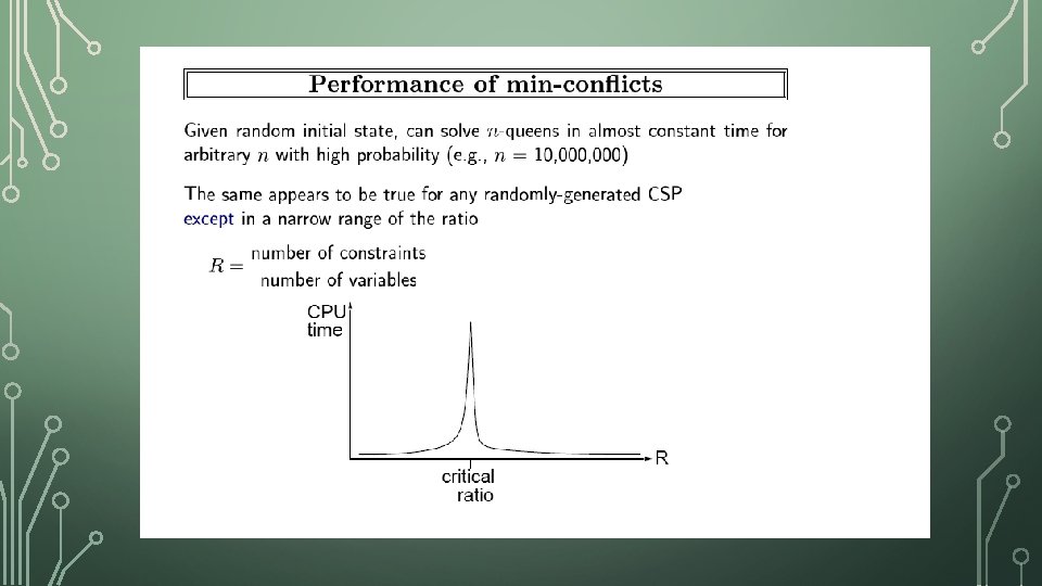
ADVANTAGES OF LOCAL SEARCH • Local search can be particularly useful in an online setting • Airline schedule example • • E. g. , mechanical problems require that 1 plane is taken out of service Can locally search for another “close” solution in state-space Much better (and faster) in practice than finding an entirely new schedule The runtime of min-conflicts is roughly independent of problem size. • • Can solve the millions-queen problem in roughly 50 steps. Why? • n-queens is easy for local search because of the relatively high density of solutions in state-space

HILL CLIMBING PROBLEMS

HILL CLIMBING QUIZ Starting from X, where do you end up ? Starting from Y, where do you end up ? Starting from Z, where do you end up ?

SIMULATED ANNEALING • Idea: Escape local maxima by allowing random downhill moves • But make them rarer as time goes on 64

STRUCTURE

PROBLEM STRUCTURE • Extreme case: independent subproblems • Example: Tasmania and mainland do not interact • Independent subproblems are identifiable as connected components of constraint graph • Suppose a graph of n variables can be broken into subproblems of only c variables: • • Worst-case solution cost is O((n/c)(dc)), linear in n E. g. , n = 80, d = 2, c =20 280 = 4 billion years at 10 million nodes/sec (4)(220) = 0. 4 seconds at 10 million nodes/sec

TREE-STRUCTURED CSPS • • • Theorem: • if a constraint graph has no loops then the CSP can be solved in O(nd 2) time • linear in the number of variables! Compare difference with general CSP, where worst case is O(d n) This property also applies to probabilistic reasoning (later): an example of the relation between syntactic restrictions and the complexity of reasoning

ALGORITHM FOR SOLVING TREE-STRUCTURED CSPS • Choose some variable as root, order variables from root to leaves such that every node’s parent precedes it in the ordering. • • • Every variable now has 1 parent Backward Pass • • • Label variables from X 1 to Xn) For j from n down to 2, apply arc consistency to arc [Parent(Xj), Xj) ] Remove values from Parent(Xj) if needed Forward Pass • For j from 1 to n assign Xj consistently with Parent(Xj )

Backward Pass TREE-STRUCTURED CSPS

TREE-STRUCTURED CSPS Backward Pass Start from F. Parent is D. Is D F consistent? No we need to remove from D.

Next look at E. Parent is D. Is D E consistent? Yes No need to remove a value from D. Next consider B D. It is also consistent. Next: B C. Not consistent; need to remove from B.

Finally consider A B. But, now A B is not arc consistent. Need to remove from A. Note that we moved backwards and touched each arc just once to make them consistent. Now we will move forward from A and make value assignments.

Forward Pass A is already red. There is only one value for B: blue. B C: only one value for C: green. B D: two possible values. Let’s pick green. D E: to stay consistent, must pick blue for E. D F: only one value for F: blue. Note that at each step forward, we were guaranteed to have a consistent value assignment because in the backward direction we ensured arc consistency for each arc. This allowed us to solve the problem in linear time.

TREE CSP COMPLEXITY • Backward pass • n arc checks • Each has complexity d 2 at worst • Forward pass • n variable assignments, O(nd) Overall complexity is O(nd 2) Algorithm works because if the backward pass succeeds, then every variable by definition has a legal assignment in the forward pass

WHAT ABOUT NON-TREE CSPS? • General idea is to convert the graph to a tree • Two general approaches • Assign values to specific variables (Cutset method) • Construct a tree-decomposition of the graph

NEARLY TREE-STRUCTURED CSPS • Conditioning: instantiate a variable, prune its neighbors' domains • Cutset conditioning: instantiate (in all ways) a set of variables such that the remaining constraint graph is a tree • Cutset size c gives runtime O( (dc) (n-c) d 2 ), very fast for small c

CUTSET CONDITIONING ALGORITHM • Choose a subset S of variables from the graph so that graph without S is a tree • S = “cutset” • For each possible consistent assignment for S • Remove any inconsistent values from remaining variables that are inconsistent with S • Use tree-structured CSP to solve the remaining tree-structure • • If it has a solution, return it along with S If not, continue to try other assignments for S

CUTSET CONDITIONING Choose a cutset SA Instantiate the cutset (all possible ways) SA Compute residual CSP for each assignment Solve the residual CSPs (tree structured) SA SA

FINDING THE OPTIMAL CUTSET • If c is small, this technique works very well • However, finding smallest cutset is NP-hard • But there are good approximation algorithms

CUTSET QUIZ • Find the smallest cutset for the graph below.

TREE DECOMPOSITIONS

TREE DECOMPOSITION • Idea: create a tree-structured graph of mega-variables • Each mega-variable encodes part of the original CSP • Subproblems overlap to ensure consistent solutions M 1 {(WA=r, SA=g, NT=b), (WA=b, SA=r, NT=g), …} Q SA {(NT=r, SA=g, Q=b), (NT=b, SA=g, Q=r), …} shared vars SA Q NS W SA shared vars NT M 4 Agree on NT M 3 Agree on WA M 2 NS W V SA Agree: (M 1, M 2) {((WA=b, SA=r, NT=g), (NT=g, SA=r, Q=b)), …}

RULES FOR A TREE DECOMPOSITION • Every variable appears in at least one of the subproblems • If two variables are connected in the original problem, they must appear together (with the constraint) in at least one subproblem • If a variable appears in two subproblems, it must appear in each node on the path.

TREE DECOMPOSITION ALGORITHM • View each subproblem as a “super-variable” • Domain = set of solutions for the subproblem • Obtained by running a CSP on each subproblem • E. g. , 6 solutions for 3 fully connected variables in map problem • Now use the tree CSP algorithm to solve the constraints connecting the subproblems • Declare a subproblem a root node, create tree • Backward and forward passes • Example of “divide and conquer” strategy