CSC 458 Data Analytics I Minimum Description Length

CSC 458– Data Analytics I, Minimum Description Length, and Evaluating Numeric Prediction November 2017 Dr. Dale Parson Read chapters 5. 8 & 5. 9 in the 3 rd Edition Weka textbook, 5. 9 & 5. 10 in the 4 th Edition.

MDL principle (textbook 5. 9 3 rd ed. , or 5. 10 4 th ed. ) • MDL stands for minimum description length • The description length is defined as: space required to describe a theory + space required to describe theory’s mistakes • In our case theory is the classifier and the mistakes are the errors on the training data • Aim: we seek a classifier with minimal DL • MDL principle is a model selection criterion • Enables us to choose a classifier of an appropriate complexity to combat overfitting 2

Model selection criteria • Model selection criteria attempt to find a good compromise between: • The complexity of a model • Its prediction accuracy on the training data • Reasoning: a good model is a simple model that achieves high accuracy on the given data • Also known as Occam’s Razor : the best theory is the smallest one that describes all the facts William of Ockham, born in the village of Ockham in Surrey (England) about 1285, was the most influential philosopher of the 14 th century and a controversial theologian. 3

Elegance vs. errors • • Theory 1: very simple, elegant theory that explains the data almost perfectly Theory 2: significantly more complex theory that reproduces the data without mistakes Theory 1 is probably preferable Classical example: Kepler’s three laws on planetary motion • Less accurate than Copernicus’s latest refinement of the Ptolemaic theory of epicycles on the data available at the time 4

MDL and compression • MDL principle relates to data compression: • The best theory is the one that compresses the data the most • In supervised learning, to compress the labels of a dataset, we generate a model and then store the model and its mistakes • We need to compute (a) the size of the model, and (b) the space needed to encode the errors • (b) easy: use the informational loss function • (a) need a method to encode the model 5

Evaluating Numeric Prediction Section 5. 8 in the older textbook, 3 rd edition. Section 5. 9 in the newer, 4 th edition.

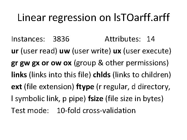
Linear regression on ls. TOarff Instances: 3836 Attributes: 14 ur (user read) uw (user write) ux (user execute) gr gw gx or ow ox (group & other permissions) links (links into this file) chlds (links to children) ext (file extension) ftype (r regular, d directory, l symbolic link, p pipe) fsize (file size in bytes) Test mode: 10 -fold cross-validation

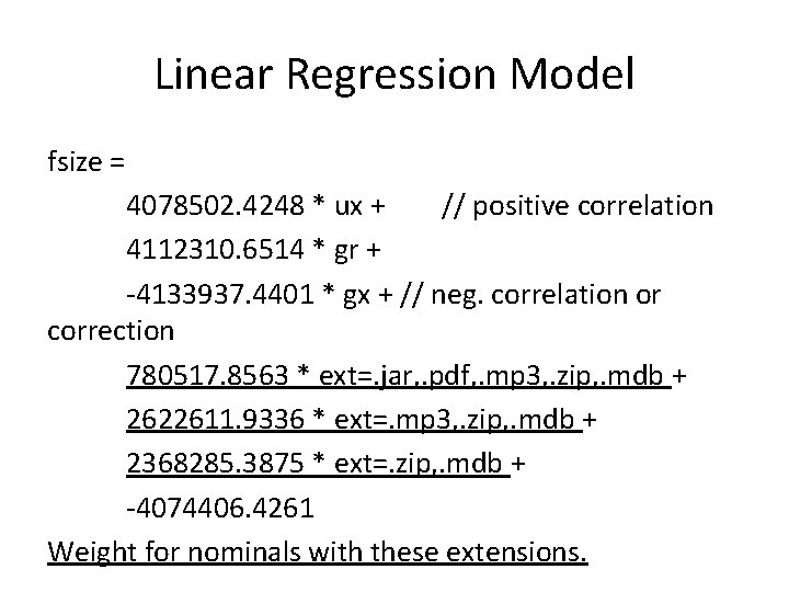
Linear Regression Model fsize = 4078502. 4248 * ux + // positive correlation 4112310. 6514 * gr + -4133937. 4401 * gx + // neg. correlation or correction 780517. 8563 * ext=. jar, . pdf, . mp 3, . zip, . mdb + 2622611. 9336 * ext=. mp 3, . zip, . mdb + 2368285. 3875 * ext=. zip, . mdb + -4074406. 4261 Weight for nominals with these extensions.

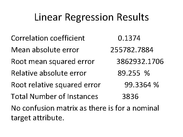
Linear Regression Results Correlation coefficient 0. 1374 Mean absolute error 255782. 7884 Root mean squared error 3862932. 1706 Relative absolute error 89. 255 % Root relative squared error 99. 3364 % Total Number of Instances 3836 No confusion matrix as there is for a nominal target attribute.

Correlation Coefficient • Correlation coefficient range: -1 through 1. • 1 is a perfect correlation. The target attribute varies linearly with the predicting attribute. • -1 is a perfect inverse correlation. The target attribute varies linearly with the predicting attribute in the opposite direction. • 0 == no correlation between the attributes.

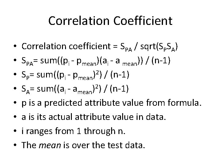
Correlation Coefficient • • Correlation coefficient = SPA / sqrt(SPSA) SPA= sum((pi - pmean)(ai - a mean)) / (n-1) SP= sum((pi - pmean)2) / (n-1) SA= sum((ai - amean)2) / (n-1) p is a predicted attribute value from formula. a is its actual attribute value in data. i ranges from 1 through n. The mean is over the test data.

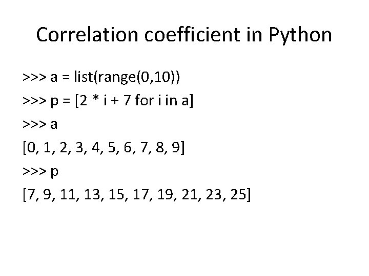
Correlation coefficient in Python >>> a = list(range(0, 10)) >>> p = [2 * i + 7 for i in a] >>> a [0, 1, 2, 3, 4, 5, 6, 7, 8, 9] >>> p [7, 9, 11, 13, 15, 17, 19, 21, 23, 25]

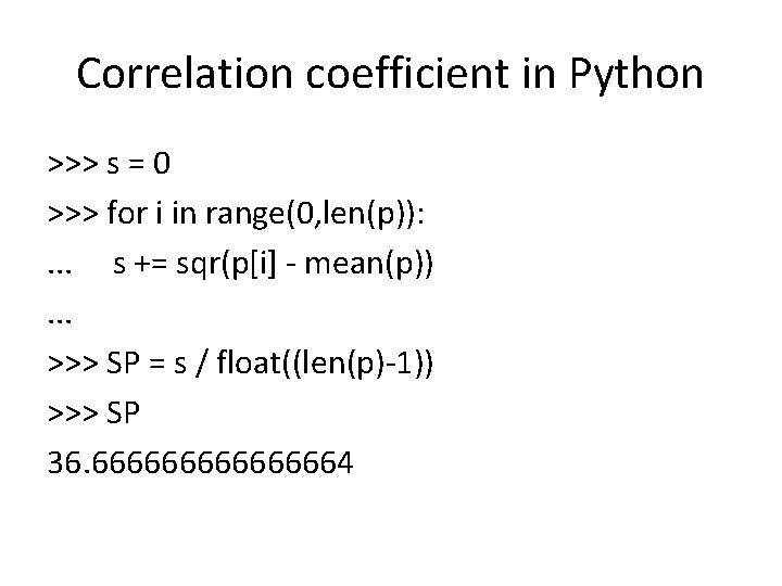
Correlation coefficient in Python >>> s = 0 >>> for i in range(0, len(p)): . . . s += sqr(p[i] - mean(p)). . . >>> SP = s / float((len(p)-1)) >>> SP 36. 66666664

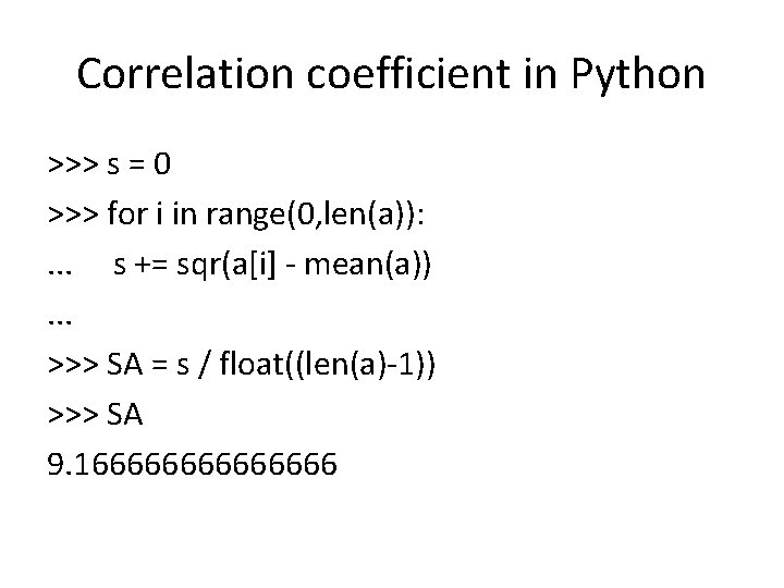
Correlation coefficient in Python >>> s = 0 >>> for i in range(0, len(a)): . . . s += sqr(a[i] - mean(a)). . . >>> SA = s / float((len(a)-1)) >>> SA 9. 16666666

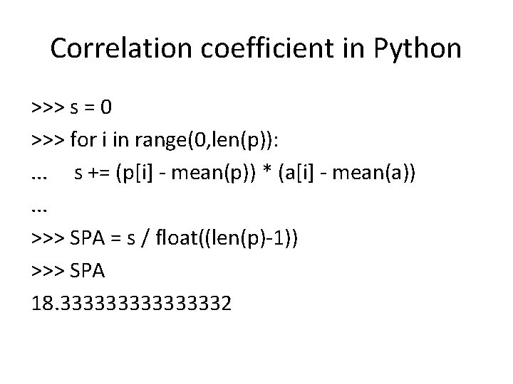
Correlation coefficient in Python >>> s = 0 >>> for i in range(0, len(p)): . . . s += (p[i] - mean(p)) * (a[i] - mean(a)). . . >>> SPA = s / float((len(p)-1)) >>> SPA 18. 33333332

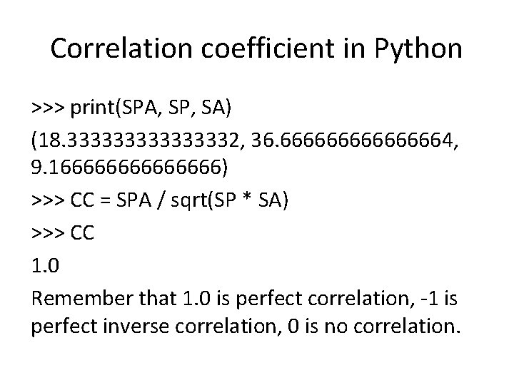
Correlation coefficient in Python >>> print(SPA, SP, SA) (18. 33333332, 36. 66666664, 9. 16666666) >>> CC = SPA / sqrt(SP * SA) >>> CC 1. 0 Remember that 1. 0 is perfect correlation, -1 is perfect inverse correlation, 0 is no correlation.

Linear Regression Results Correlation coefficient 0. 1374 Mean absolute error 255782. 7884 Root mean squared error 3862932. 1706 Relative absolute error 89. 255 % Root relative squared error 99. 3364 % Total Number of Instances 3836 No confusion matrix as there is for a nominal target attribute.

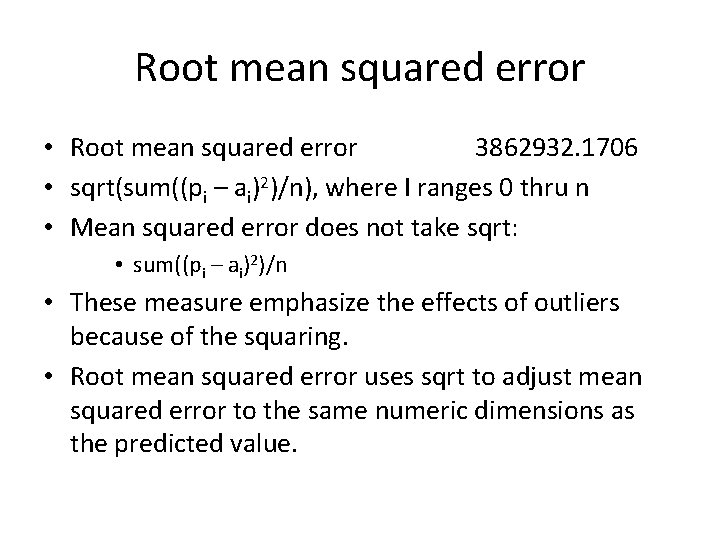
Root mean squared error • Root mean squared error 3862932. 1706 • sqrt(sum((pi – ai)2)/n), where I ranges 0 thru n • Mean squared error does not take sqrt: • sum((pi – ai)2)/n • These measure emphasize the effects of outliers because of the squaring. • Root mean squared error uses sqrt to adjust mean squared error to the same numeric dimensions as the predicted value.

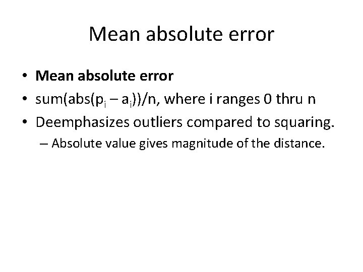
Mean absolute error • sum(abs(pi – ai))/n, where i ranges 0 thru n • Deemphasizes outliers compared to squaring. – Absolute value gives magnitude of the distance.

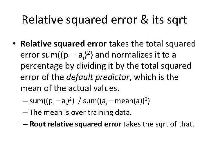
Relative squared error & its sqrt • Relative squared error takes the total squared error sum((pi – ai)2) and normalizes it to a percentage by dividing it by the total squared error of the default predictor, which is the mean of the actual values. – sum((pi – ai)2) / sum((ai – mean(a))2) – The mean is over training data. – Root relative squared error takes the sqrt of that.

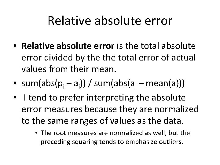
Relative absolute error • Relative absolute error is the total absolute error divided by the total error of actual values from their mean. • sum(abs(pi – ai)) / sum(abs(ai – mean(a))) • I tend to prefer interpreting the absolute error measures because they are normalized to the same ranges of values as the data. • The root measures are normalized as well, but the preceding squaring tends to emphasize outliers.

Linear Regression Results Correlation coefficient 0. 1374 Mean absolute error 255782. 7884 Root mean squared error 3862932. 1706 Relative absolute error 89. 255 % Root relative squared error 99. 3364 % Total Number of Instances 3836 No confusion matrix as there is for a nominal target attribute.