CS 775 Advanced Pattern Recognition Slide set 1

CS 775: Advanced Pattern Recognition Slide set 1 Daniel Barbará

Chapter 1 Introduction to Pattern Recognition (Sections 1. 1 -1. 6 DHS)

Machine Perception n Build a machine that can recognize patterns: – Speech recognition – Fingerprint identification – OCR (Optical Character Recognition) – DNA sequence identification

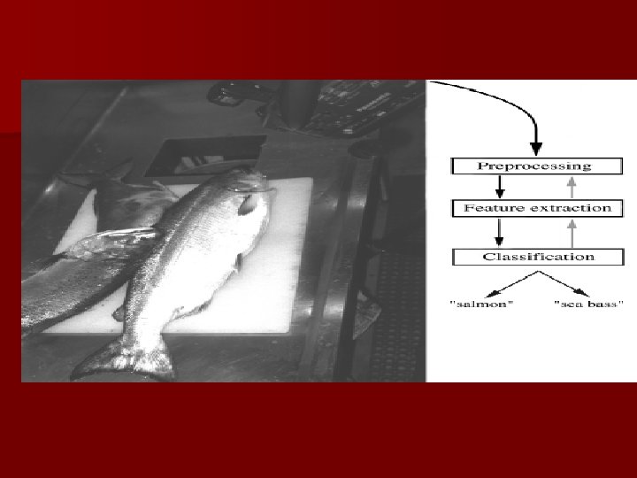
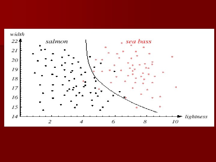
An Example n “Sorting incoming Fish on a conveyor according to species using optical sensing” Sea bass Species Salmon

n Problem Analysis – Set up a camera and take some sample images to extract features § Length § Lightness § Width § Number and shape of fins § Position of the mouth, etc… § This is the set of all suggested features to explore for

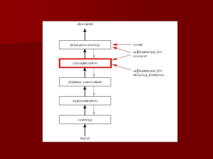
n Preprocessing – Use a segmentation operation to isolate fishes from one another and from the background n Information from a single fish is sent to a feature extractor whose purpose is to reduce the data by measuring certain features n The features are passed to a classifier

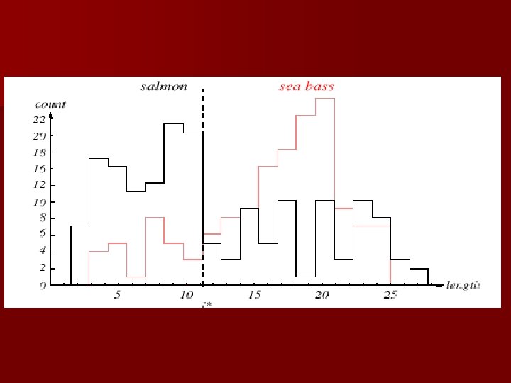
n Classification – Select the length of the fish as a possible feature for discrimination

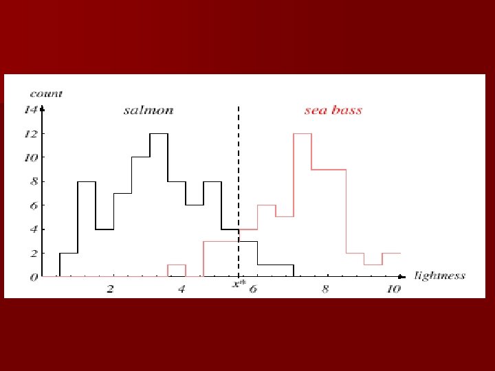
The length is a poor feature alone! Select the lightness as a possible feature.

n Threshold decision boundary and cost relationship – Move our decision boundary toward smaller values of lightness in order to minimize the cost (reduce the number of sea bass that are classified salmon!) Task of decision theory

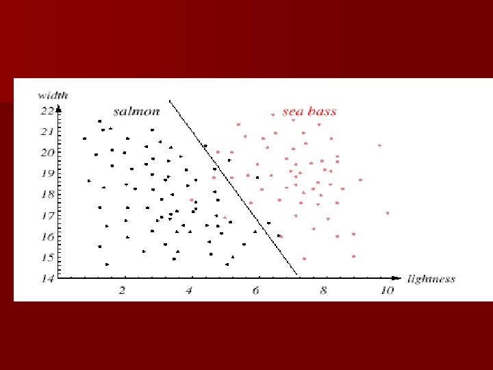
n Adopt the lightness and add the width of the fish Fish x. T = [x 1 , x 2 ] Lightness Width

n We might add other features that are not correlated with the ones we already have. A precaution should be taken not to reduce the performance by adding such “noisy features” n Ideally, the best decision boundary should be the one which provides an optimal performance such as in the following figure:

n However, our satisfaction is premature because the central aim of designing a classifier is to correctly classify novel input Issue of generalization!

Pattern Recognition Systems n Sensing – Use of a transducer (camera or microphone) – PR system depends of the bandwidth, the resolution sensitivity distortion of the transducer n Segmentation and grouping – Patterns should be well separated and should

Learning and Adaptation n Supervised learning – A teacher provides a category label or cost for each pattern in the training set n Unsupervised learning – The system forms clusters or “natural groupings” of the input patterns

Conclusion n Reader seems to be overwhelmed by the number, complexity and magnitude of the sub-problems of Pattern Recognition n Many of these sub-problems can indeed be solved n Many fascinating unsolved problems still remain

Chapter 2 DHS (Part 1): Bayesian Decision Theory (Sections 2. 1 -2. 2) Introduction Bayesian Decision Theory–Continuous Features

Basic problem a machine capable of assigning x to one of many classes (w 1, w 2, …, wc) n Supervised learning: you are given a series of examples (xi, yi) where yi is one of wk n Produce

Inference and Decision Three distinct approaches to solve decision problems 1. Solve the inference problem determining P(x|wi) for each class. Apply Bayes to get P(wi|x). GENERATIVE MODELS 2. Solve the inference problem by determining P(wi|x) directly. DISCRIMINATIVE MODELS 3. Find a function f(x) –called discriminant function- which maps each input into a class label 1 and 2 are followed by the use of DECISION THEORY

Introduction n The sea bass/salmon example – State of nature, prior § State of nature is a random variable § The catch of salmon and sea bass is equiprobable – P( 1) = P( 2) (uniform priors) – P( 1) + P( 2) = 1 (exclusivity and exhaustivity)

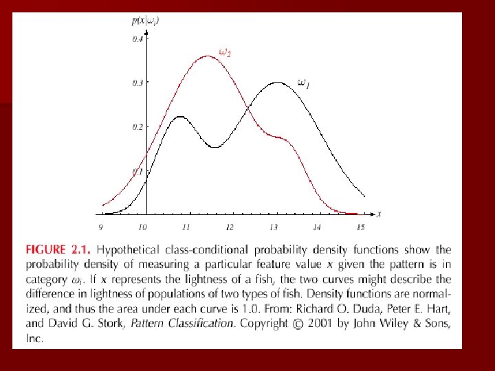
n Decision rule with only the prior information – Decide 1 if P( 1) > P( 2) otherwise decide 2 n Use of the class –conditional information n P(x | 1) and P(x | 2) describe the difference in lightness between populations of sea and salmon

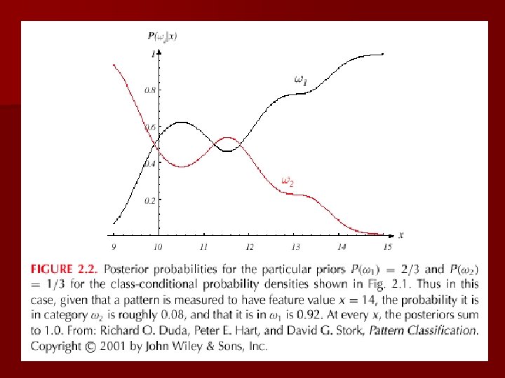
n Posterior, likelihood, evidence Bayes – P( j | x) = P(x | j). P ( j) / P(x) – Where in case of two categories – Posterior = (Likelihood. Prior) / Evidence

Minimum Misclassification Rate

n Decision given the posterior probabilities X is an observation for which: if P( 1 | x) > P( 2 | x) nature = 1 if P( 1 | x) < P( 2 | x) nature = 2 True state of Therefore: whenever we observe a particular x, the probability of error is :

n Minimizing the probability of error n Decide 1 if P( 1 | x) > P( 2 | x); otherwise decide 2 Therefore: x)] Cannot do better than this! P(error | x) = min [P( 1 | x), P( 2 | (Bayes decision)

Bayesian Decision Theory – Continuous Features n Generalization of the preceding ideas – Use of more than one feature – Use more than two states of nature – Allowing actions and not only decide on the state of nature – Introduce a loss of function which is more general than the probability of error

n Allowing actions other than classification primarily allows the possibility of rejection n Refusing cases! n The to make a decision in close or bad loss function states how costly each action taken is

Reject Option

Let { 1, 2, …, c} be the set of c states of nature (or “categories”) Let { 1, 2, …, a} be the set of possible actions Let ( i | j) be the loss incurred for taking action i when the state of nature is j

Overall risk R = Sum of all R( i | x) for i = 1, …, a Conditional risk Minimizing R 1, …, a Minimizing R( i | x) for i = 1, …, a

Select the action i for which R( i | x) is minimum R is minimum and R in this case is called the Bayes risk = best performance that can be achieved!

n Two-category classification 1 : deciding 1 2 : deciding 2 ij = ( i | j) loss incurred for deciding i when the true state of nature is j Conditional risk: R( 1 | x) = 11 P( 1 | x) + 12 P( 2 | x) R( 2 | x) = 21 P( 1 | x) + 22 P( 2 | x)

Our rule is the following: if R( 1 | x) < R( 2 | x) action 1: “decide 1” is taken This results in the equivalent rule : decide 1 if: ( 21 - 11) P(x | 1) P( 1) > ( 12 - 22) P(x | 2) P( 2) and decide 2 otherwise

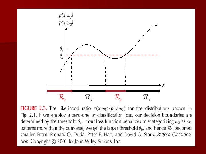
Likelihood ratio: Likelihood ratio The preceding rule is equivalent to the following rule: Then take action 1 (decide 1) Otherwise take action 2 (decide 2)

Optimal decision property “If the likelihood ratio exceeds a threshold value independent of the input pattern x, we can take optimal actions”

Exercise Select the optimal decision where: W = { 1 , 2 } P(x | 1) N(2, 0. 5) (Normal P(x | 2) N(1. 5, 0. 2) distribution) P( 1) = 2/3 P( 2) = 1/3

Chapter 2 (Part 2): Bayesian Decision Theory (Sections 2. 3 -2. 5) Minimum-Error-Rate Classification Classifiers, Discriminant Functions and Decision Surfaces The Normal Density

Minimum-Error-Rate Classification n Actions are decisions on classes If action i is taken and the true state of nature is j then: the decision is correct if i = j and in error if i j n Seek a decision rule that minimizes the probability of error which is the error rate

n Introduction of the zero-one loss function: Therefore, the conditional risk is: “The risk corresponding to this loss function is the average probability error”

the risk requires maximize P( i | x) (since R( i | x) = 1 – P( i | x)) n Minimize n For Minimum error rate – Decide i if P ( i | x) > P( j | x) j i

n Regions of decision and zero-one loss function, therefore: n If is the zero-one loss function which means:

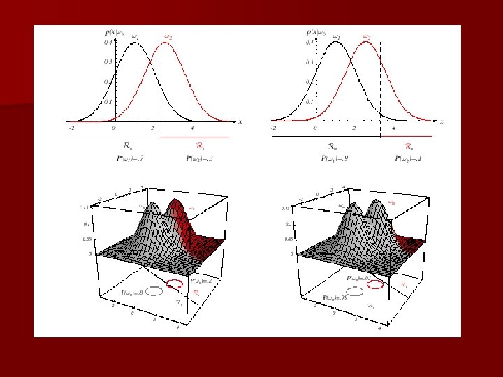
Minimax Criterion n The prior probabilities might vary widely and in an unpredictable way n We want to use the classifier elsewhere and we don’t know the priors well there n Design our classifier so that the worst overall risk is as small as possible: minimize the maximum possible overall risk

Minmax Risk =0 for minmax solution

MINMAX RISK

Minmax solution

Why Separate Inference and Decision? n n Minimizing risk (loss matrix may change over time) Reject option Unbalanced class priors Combining models

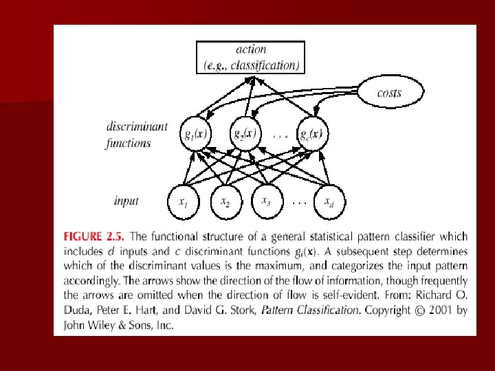
Classifiers, Discriminant Functions and Decision Surfaces n The multi-category case – Set of discriminant functions gi(x), i = 1, …, c – The classifier assigns a feature vector x to class i if: gi(x) > gj(x) j i

n Let gi(x) = - R( i | x) (max. discriminant corresponds to min. risk!) n For the minimum error rate, we take gi(x) = P( i | x) (max. discrimination corresponds to max. posterior!) gi(x) P(x | i) P( i) gi(x) = ln P(x | i) + ln P( i) (ln: natural logarithm!)

n Feature space divided into c decision regions if gi(x) > gj(x) j i then x is in Ri (Ri means assign x to i) n The two-category case – A classifier is a “dichotomizer” that has two discriminant functions g 1 and g 2 Let g(x) g 1(x) – g 2(x) Decide 1 if g(x) > 0 ; Otherwise decide 2

– The computation of g(x)

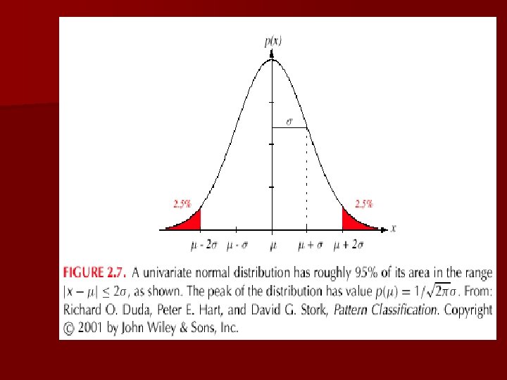
The Normal Density n Univariate density – – Density which is analytically tractable Continuous density A lot of processes are asymptotically Gaussian Handwritten characters, speech sounds are ideal or prototype corrupted by random process (central limit theorem) Where: = mean (or expected value) of x 2 = expected squared deviation or variance

n Multivariate density – Multivariate normal density in d dimensions is: where: x = (x 1, x 2, …, xd)t vector form) (t stands for the transpose = ( 1, 2, …, d)t mean vector = d*d covariance matrix | | and -1 are determinant and inverse respectively

Chapter 2 (part 3) Bayesian Decision Theory (Sections 2 -6, 2 -9) Discriminant Functions for the Normal Density Bayes Decision Theory – Discrete Features

Discriminant Functions for the Normal Density n We saw that the minimum error-rate classification can be achieved by the discriminant function gi(x) = ln P(x | i) + ln P( i) n Case of multivariate normal

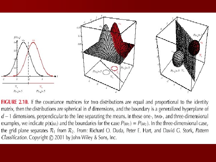
n Case i = 2. I (I stands for the identity matrix)

– A classifier that uses linear discriminant functions is called “a linear machine” – The decision surfaces for a linear machine are pieces of hyperplanes defined by: gi(x) = gj(x)

– The hyperplane separating Ri and Rj always orthogonal to the linking the means!

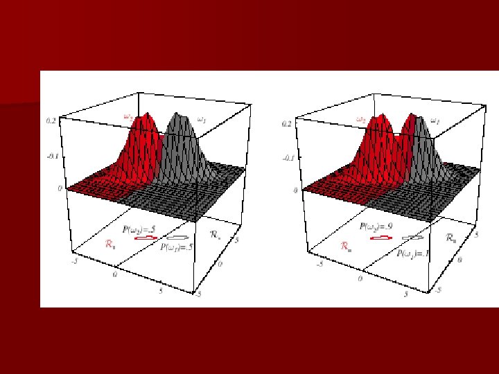
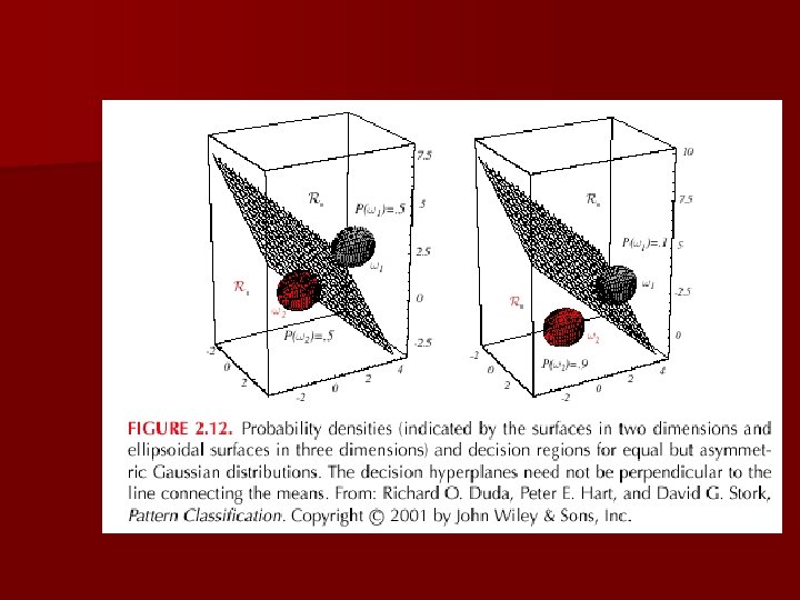
i = (covariance of all classes are identical but arbitrary!) n Case – Hyperplane separating Ri and Rj (the hyperplane separating Ri and Rj is generally not orthogonal to the line between the means!)

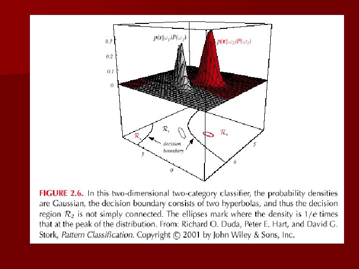
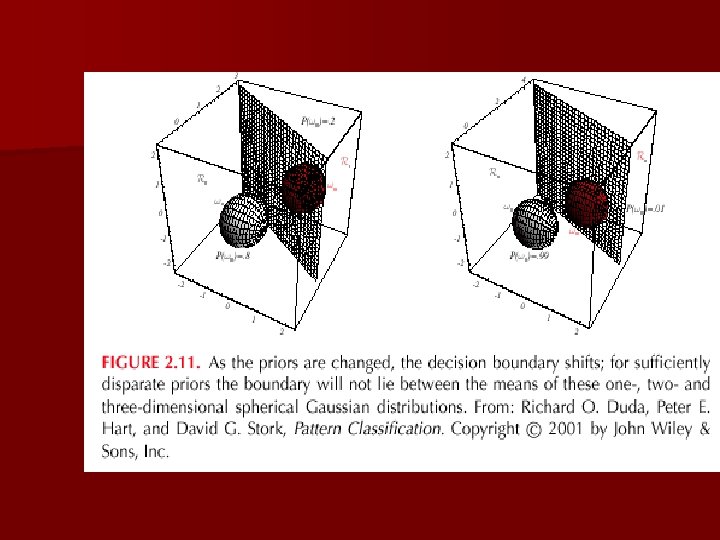
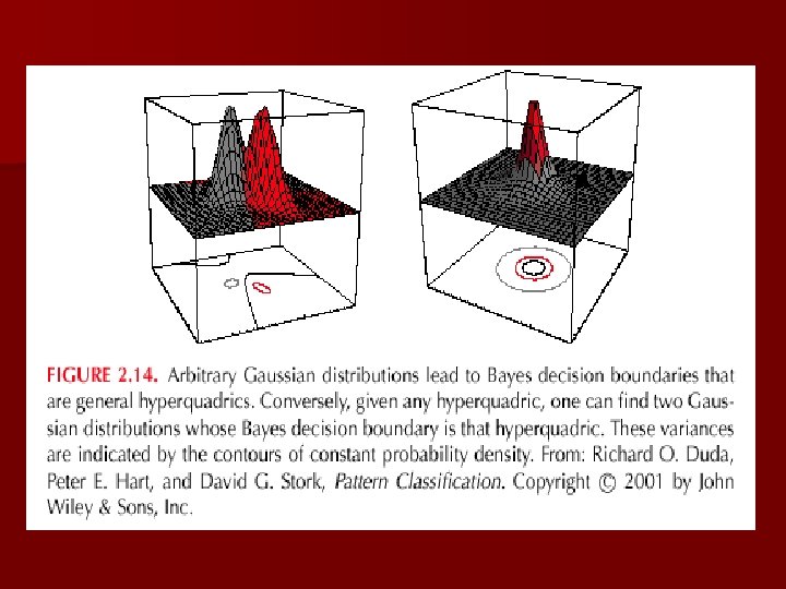
n Case i = arbitrary – The covariance matrices are different for each category (Hyperquadrics which are: hyperplanes, pairs of hyperplanes, hyperspheres, hyperellipsoids, hyperparaboloids, hyperboloids)

Bayes Decision Theory – Discrete Features n Components of x are binary or integer valued, x can take only one of m discrete values v 1, v 2, …, vm n Case of independent binary features in 2 category problem Let x = [x 1, x 2, …, xd ]t where each xi is either 0 or 1, with probabilities: pi = P(xi = 1 | 1) qi = P(xi = 1 | 2)

n The discriminant function in this case is: