CS 686 Configuration Space II SungEui Yoon Course

CS 686: Configuration Space II Sung-Eui Yoon (윤성의) Course URL: http: //sgvr. kaist. ac. kr/~sungeui/MPA

Class Objectives ● Configuration space ● ● 2 Definitions and examples Obstacles Paths Metrics

Obstacles in the Configuration Space ● A configuration q is collision-free, or free, if a moving object placed at q does not intersect any obstacles in the workspace ● The free space F is the set of free configurations ● A configuration space obstacle (C-obstacle) is the set of configurations where the moving object collides with workspace obstacles 3

Disc in 2 -D Workspace workspace 4 configuration space

Polygonal Robot Translating & Rotating in 2 -D Workspace obstacle 5 C-space

Polygonal Robot Translating & Rotating in 2 -D Workspace 6 C-space

Polygonal Robot Translating & Rotating in 2 -D Workspace … 3 D C-space 7

C-Obstacle Construction ● Input: ● Polygonal moving object translating in 2 -D workspace ● Polygonal obstacles ● Output: ● Configuration space obstacles represented as polygons 8

Minkowski Sum ● The Minkowski sum of two sets P and Q, denoted by P Q, is defined as P Q = { p+q | p P, q Q } wiki 9 ● Similarly, the Minkowski difference is defined as P – Q = { p–q | p P, q Q } = P + -Q

Minkowski Sum of Convex Polygons ● The Minkowski sum of two convex polygons P and Q of m and n vertices respectively is a convex polygon P + Q of m + n vertices. ● The vertices of P + Q are the “sums” of vertices of P and Q. wiki 10

Observation ● Suppose P is an obstacle in the workspace and M is a moving object ● Then the C-obstacle is P – M m P p o 11 M

Computing C-obstacles 12

Computational efficiency ● Running time O(n+m) ● Space O(n+m) ● Non-convex obstacles ● Decompose into convex polygons (e. g. , triangles or trapezoids), compute the Minkowski sums, and take the union ● Complexity of Minkowksi sum O(n 2 m 2) ● 3 -D workspace ● Convex case: O(nm) ● Non-convex case: O(n 3 m 3) 13

Worst case example ● O(n 2 m 2) complexity 2 D example Agarwal et al. 02 14

444 tris 15 1, 134 tris

Union of 66, 667 primitives

Main Message ● Computing the free or obstacle space in an accurate way is an expensive and nontrivial problem ● Lead to many sampling based methods ● Locally utilize many geometric concepts developed for designing complete planners 17

Approximation of Configuration Free Space ● Dancing PRM* : Simultaneous Planning of Sampling and Optimization with Configuration Free Space Approximation ● Approximate C-Space and perform planning ● Improve the quality in an iterative manner Video 18

Velodyne 21

Kinect and Xtion ● Kinect resolution ● 640× 480 pixels @ 30 Hz (RGB camera) ● 640× 480 pixels @ 30 Hz (IR depth-finding camera) 22

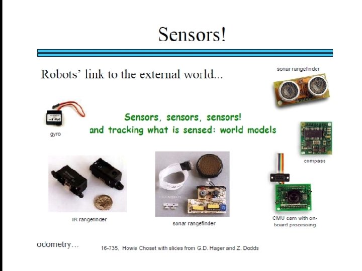
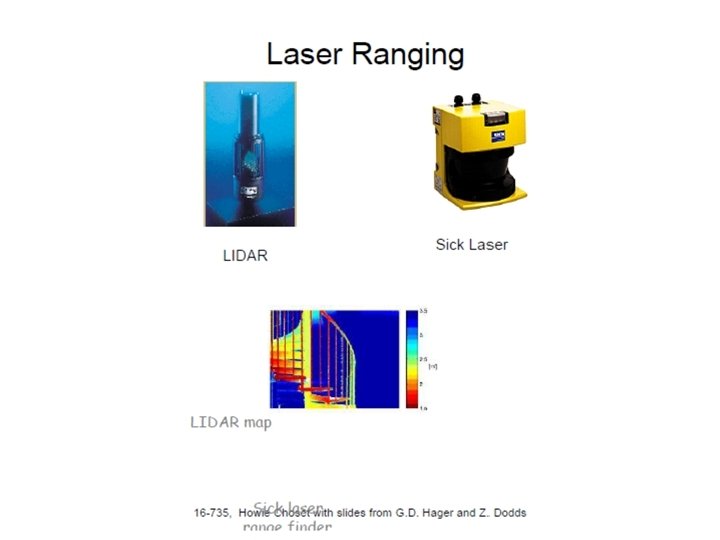
Whole Picture ● Sensor ● Point clouds as obstacle map ● Control ● Compute force controls given a computed path ● SLAM (Simultaneous Localization and Mapping) ● Path/motion planner 23

Configuration space ● Definitions and examples ● Obstacles ● Paths ● Metrics 24

Paths in the configuration space workspace configuration space ● A path in C is a continuous curve connecting two configurations q and q’ : such that t(0) = q and t(1)=q’. 25

Constraints on paths ● A trajectory is a path parameterized by time: ● Constraints ● Finite length ● Bounded curvature ● Smoothness ● Minimum length ● Minimum time ● Minimum energy ● … 26

Free Space Topology ● A free path lies entirely in the free space F ● The moving object and the obstacles are modeled as closed subsets, meaning that they contain their boundaries. ● One can show that the C-obstacles are closed subsets of the configuration space C as well ● Consequently, the free space F is an open subset of C 27

Semi-Free Space ● A configuration q is semi-free if the moving object placed q touches the boundary, but not the interior of obstacles. ● Free, or ● In contact ● The semi-free space is a closed subset of C 28

Example 29

Example 30

Homotopic Paths ● Two paths t and t’ (that map from U to V) with the same endpoints are homotopic if one can be continuously deformed into the other: with h(s, 0) = t(s) and h(s, 1) = t’(s). ● A homotopic class of paths contains all paths that are homotopic to one another 31

Configuration space ● Definitions and examples ● Obstacles ● Paths ● Metrics 32

Metric in Configuration Space ● A metric or distance function d in a configuration space C is a function such that ● d(q, q’) = 0 if and only if q = q’, ● d(q, q’) = d(q’, q), ●. 33

Example ● Robot A and a point x on A ● x(q): position of x in the workspace when A is at configuration q ● A distance d in C is defined by d(q, q’) = maxx A || x(q) - x(q’) ||, q 34 q’ where ||x - y|| denotes the Euclidean distance between points x and y in the workspace.

Lp Metrics ● L 2: Euclidean metric ● L 1: Manhattan metric ● L∞: Max (| xi – xi′ |) 35

Examples in R 2 x S 1 ● Consider R 2 x S 1 ● q = (x, y, q), q’ = (x’, y’, q’) with q, q’ [0, 2 p) ● a = min { |q - q’ | , 2 p - |q - q’| } q a ● d(q, q’) = sqrt( (x-x’)2 + (y-y’)2 + a 2 ) ) 36 q’

Class Objectives were: ● Configuration space ● ● 37 Definitions and examples Obstacles Paths Metrics

Summary 38

Next Time…. ● Collision detection and distance computation 39

Homework ● Submit summaries of 2 ICRA/IROS/RSS/Co. RL/TRO/IJRR papers ● Go over the next lecture slides ● Come up with 3 questions before the midterm exam 40

41

Workspace Obstacle C-space

Polygonal Robot Translating & Rotating in 2 -D Workspace … 3 D C-space 43

Disc in 2 -D Workspace 44 C-space